Chapter 5: Drilling Fluid Characterization

Learning Objectives

By the end of this chapter, you will be able to:

• Explain why continuous monitoring of drilling fluid properties is essential to safe and efficient drilling

• Describe how drilling fluid density is measured and identify the limitations of common measurement methods

• Define shear stress, shear rate, and viscosity, and explain how each is measured with a rotational viscometer

• Distinguish between Newtonian, Bingham Plastic, Power Law, and Herschel-Bulkley rheological models and identify which best describes a given drilling fluid

• Define plastic viscosity, yield point, and apparent viscosity, and calculate each from Fann viscometer readings

• Explain thixotropy, gel strength, and why gel behavior should be flat rather than progressive

• Describe the viscosifiers used in water-based and oil-based muds and explain the mechanism by which each imparts viscosity

• Explain fluid loss control, identify consequences of excessive fluid loss, and describe how fluid loss is measured

• List the chemical and solids analyses performed on a mud check and explain the purpose of each

• Identify common drilling fluid contaminants and describe how they affect mud properties

---

5.1 Why Monitor Fluid Properties?

Drilling fluid properties are not static. As a well deepens, drilling mud continuously picks up drill solids, encounters formation waters with different chemistry, is exposed to changes temperature and pressure, and loses components through filtration into the formation. Without continuous monitoring, the mud engineer has no way to know whether the fluid is still fit for purpose — or whether it has drifted into a condition that could cause a wellbore problem.

The objectives of regular fluid monitoring are:

1. Establish a baseline and trend. A single data point tells you where the mud is. A series of data points over time tells you where it is going. Trending is more valuable than any individual measurement: a slow drift in density, viscosity, or fluid loss often signals a developing problem that can be corrected cheaply before it becomes expensive.

2. Identify potential hole problems and causes. Many drilling problems, stuck pipe, wellbore instability, lost circulation, differential sticking, manifest first as changes in mud properties. A sudden increase in low-gravity solids may indicate a reactive formation is breaking down and contaminating the mud. An unexplained density drop may indicate an influx.

3. Solve problems through fluid adjustments. Once a problem is identified, the drilling fluid is often the most direct lever available. Adjusting mud weight, viscosity, fluid loss, or inhibition chemistry can stabilize a problematic wellbore more quickly and cheaply than any mechanical intervention.

4. Prevent problems from starting. The best outcome is that careful monitoring catches trends early enough that corrective action is taken before any operational impact occurs.

Mud checks are typically performed every 4–8 hours on active drilling operations. The suite of measurements taken constitutes a mud report, which is transmitted to the operator’s office and reviewed by the drilling engineer as part of real-time well monitoring.

5.1.1 Where to Take a Sample

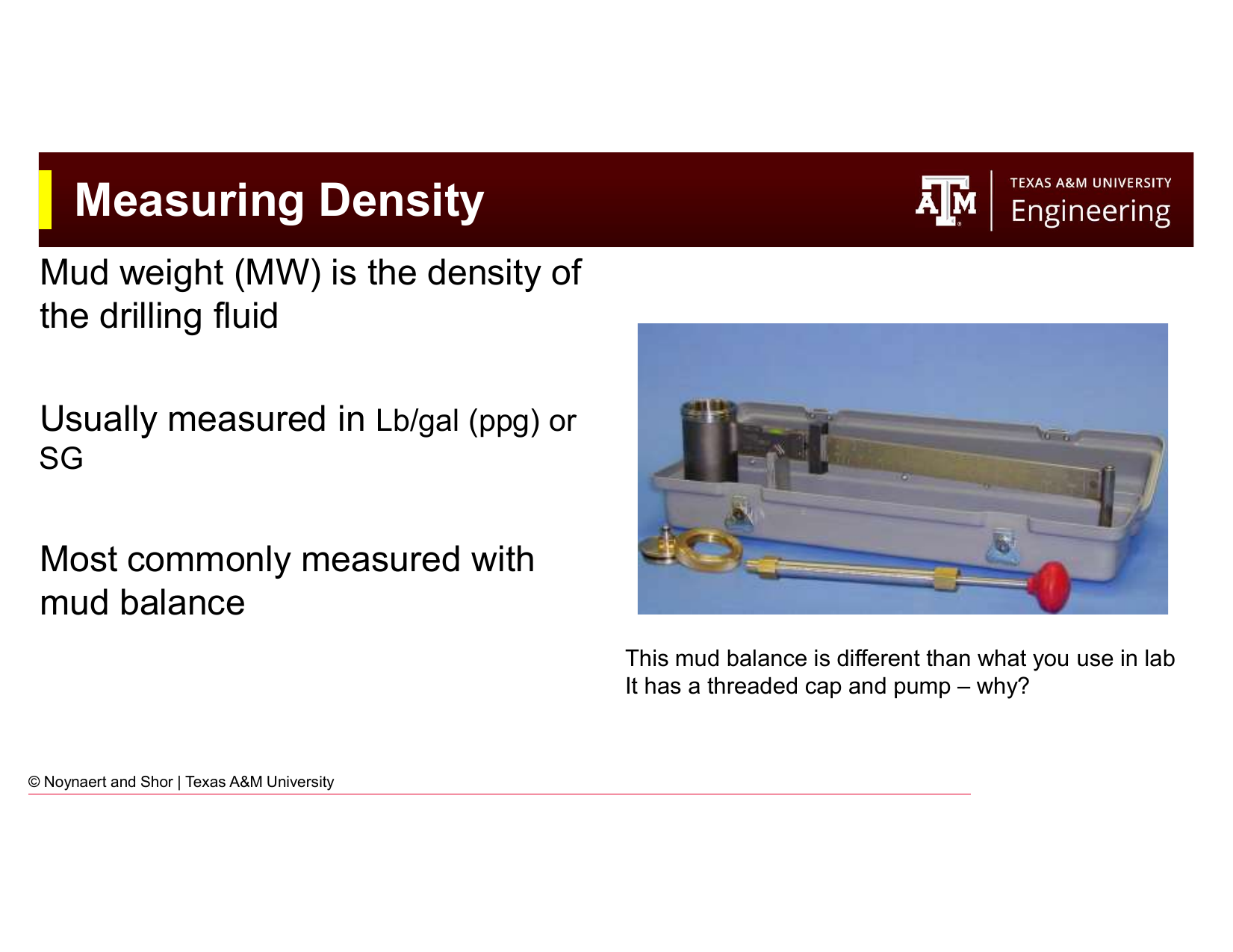
Fig. 45 Possible sample locations in the surface mud system. The choice of sample point significantly affects what the measurement tells you about the mud circulating in the hole.

Where the mud sample is taken matters. The mud circulating system has multiple points where a sample could be collected: the suction pit (before the pump), the return flow line (as mud comes back from the well), or the active pit. Each location provides different information:

• Return flow line — represents the mud as it arrives from downhole, including any gas or formation fluids it has picked up. Best for detecting contamination or influx.

• Active pit (suction) — represents the conditioned mud that is about to be pumped downhole, after solids control processing. Most representative of the fluid providing well control.

The standard practice is to report properties on the active (suction) pit mud, since this is what is actually entering the well. However, comparing return mud properties to suction mud properties can be diagnostic: significant differences may indicate formation interactions or solids loading.

---

5.2 Density Measurement

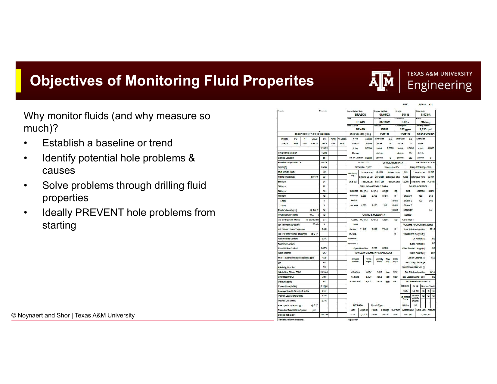
Fig. 46 The two primary properties measured in a mud check: density (mud weight) and viscosity. Density governs hydrostatic (static) pressure; viscosity governs dynamic (flowing) pressure losses.

5.2.1 The Mud Balance

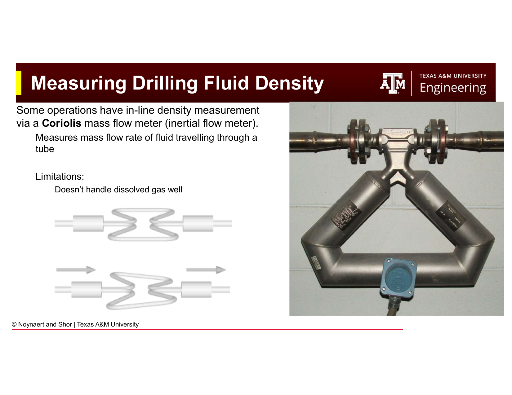
Fig. 47 A pressurized mud balance used for field density measurement. The threaded, pressurized cap allows entrapped gas bubbles to be dissolved before measurement, improving accuracy in gas-cut muds.

The standard field instrument for measuring mud density is the mud balance: a lever-arm balance in which a fixed-volume cup is filled with mud and balanced against a sliding counterweight on a graduated beam. The density is read directly from the beam position at balance.

The field mud balance is specifically designed with a threaded, pressurized cap (unlike a laboratory balance). The purpose of the pressure cap is to re-dissolve any gas bubbles that have come out of solution in the returning mud before the measurement is taken. Gas-cut mud, mud that has entrained formation gas, will read artificially low density if measured with free gas bubbles present. The pressurized cap compresses the sample, forcing the gas back into solution and giving a more accurate reading of the true mud density.

Key Term: Mud Weight

Mud weight (MW) is the density of the drilling fluid, typically expressed in pounds per gallon (ppg or lb/gal) in US oilfield units. Common equivalent expressions include specific gravity (SG) and pressure gradient (psi/ft). The conversion is:

\[\text{Pressure gradient (psi/ft)} = 0.052 \times \text{MW (ppg)}\]

\[\text{Specific Gravity (SG)} = \frac{MW (ppg)}{8.34 (ppg)}\]

5.2.2 In-Line Density Measurement: Coriolis Meter

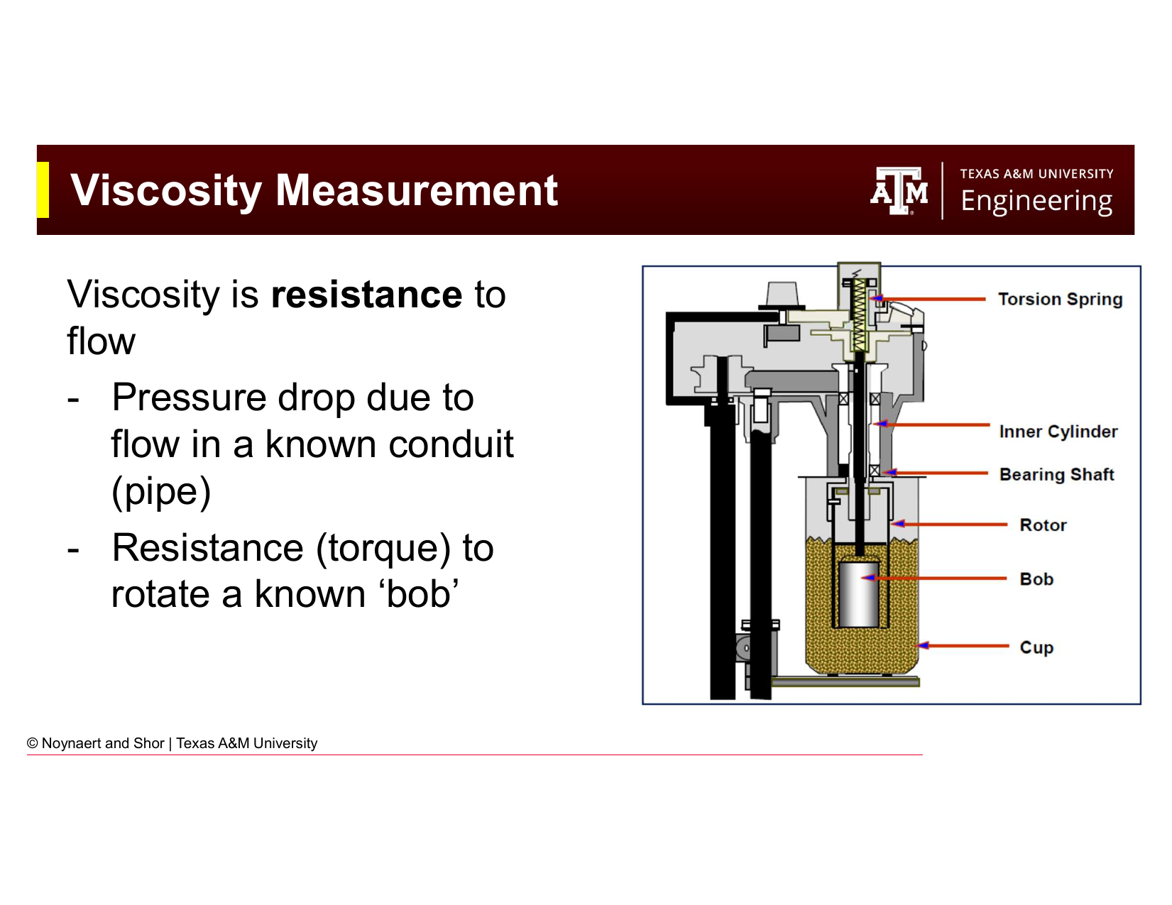
Fig. 48 A Coriolis mass flow meter for in-line mud density measurement. The meter measures mass flow rate by detecting the phase shift in vibration of a U-shaped tube caused by the Coriolis effect of the flowing fluid.

For operations requiring continuous density monitoring (such as managed pressure drilling or underbalanced drilling), a Coriolis mass flow meter can be installed in-line on the mud return line. The Coriolis meter measures the mass flow rate of the mud passing through a vibrating U-shaped tube by detecting the Coriolis-induced phase shift in the tube vibration. Density is derived from the ratio of mass flow to volumetric flow.

Limitations of Coriolis meters in drilling applications:

• Poor performance with dissolved gas — Free or dissolved gas in the returning mud disrupts the vibration signal, giving erratic or unreliable readings. This is a significant limitation since gas influx is precisely the condition where accurate density measurement is most critical.

• Low tolerance for high solids content - High solids loading (high volumes of cuttings or dissolved solids) can block the Coriolis flow meter lines and lead to inaccurate measurements.

• Cost — Coriolis meters are substantially more expensive than mud balances and require more maintenance.

---

5.3 Viscosity: Fundamentals

Before describing viscosity measurement, it is important to establish what viscosity actually is and how it is defined in engineering terms.

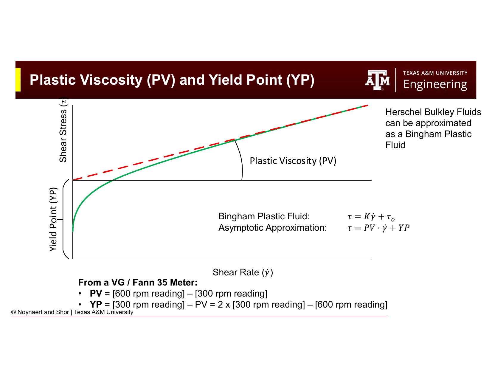
Fig. 49 The physical definitions of shear stress and shear rate in a flowing fluid. Shear stress is the force per unit area applied to the fluid; shear rate is the velocity gradient across the fluid layers. Viscosity relates the two.

Consider a fluid between two parallel plates. The lower plate is fixed; the upper plate moves at velocity \(v\). The fluid is sheared — layers closer to the moving plate move faster than layers closer to the fixed plate, producing a velocity gradient across the fluid.

Key Term: Shear Rate

Shear rate (\(\dot{\gamma}\)) is the rate of change of fluid velocity across the flow direction — the velocity gradient between adjacent layers of fluid. It is expressed in units of inverse seconds (s⁻¹):

\[\dot{\gamma} = \frac{dv}{dr}\]

In a Fann viscometer, shear rate is proportional to the rotational speed of the outer cylinder.

Conceptually, shear rate is the fluid velocity.

Key Term: Shear Stress

Shear stress (\(\tau\)) is the force per unit area required to maintain a given shear rate in the fluid. It is expressed in units of Pa or lb/100 ft². In a Fann viscometer, shear stress is proportional to the torque measured on the inner bob:

\[\tau = \frac{F}{A}\]

Conceptually, it is the amount of effort or pressure necessary to mantain the flow velocity as a particular value.

Key Term: Viscosity

Viscosity (\(\mu\)) is the fluid’s internal resistance to flow — the ratio of shear stress to shear rate. For a Newtonian fluid, viscosity is a constant independent of shear rate. For non-Newtonian fluids (including most drilling muds), the apparent viscosity depends on shear rate. Common units are centipoise (cP) or mPa·s.

Conceptually, viscosity is the ratio of effort to maintain flow to the flow velocity of a fluid.

---

5.4 Viscosity Measurement

5.4.1 The Fann VG / Fann 35 Viscometer

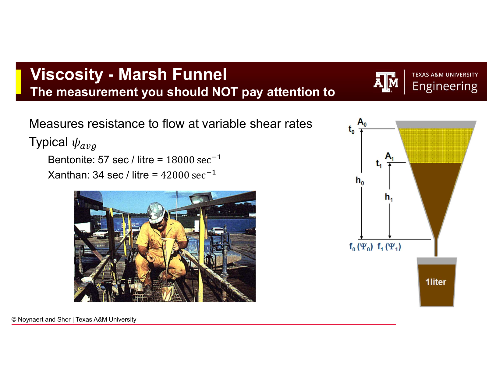
Fig. 50 The Fann VG (or equivalent Fann 35) rotational viscometer is the standard instrument for mud rheology characterization in the field and laboratory. The outer sleeve rotates at a controlled speed; the torque on the inner bob is measured as a dial reading proportional to shear stress.

The Fann VG meter (also manufactured by OFITE, Grace, and others under equivalent designations) is a coaxial cylinder (Couette) viscometer. The mud sample is placed in the annular gap between an outer rotating sleeve and a fixed inner bob. The sleeve rotates at a set speed, shearing the mud. The torque transmitted to the inner bob through the mud is measured via a calibrated spring and read from a dial.

Standard measurement speeds: 600, 300, 200, 100, 6, and 3 rpm. The dial reading at each speed is recorded as \(\theta_{600}\), \(\theta_{300}\), etc.

Unit conversions built into the instrument design:

• \(1°\text{ dial deflection} = 1.067 \text{ lb/100 ft}^2\) shear stress (approximately 1 lb/100 ft²)

• Shear rate (s⁻¹) = \(1.703 \times N\) (where \(N\) is the rotor speed in rpm)

This means:

• At 600 rpm: shear rate = 1,022 s⁻¹

• At 300 rpm: shear rate = 511 s⁻¹

• At 6 rpm: shear rate = 10.2 s⁻¹

• At 3 rpm: shear rate = 5.1 s⁻¹

Temperature standards: WBMs are tested at 120°F (49°C); OBMs at 150°F (66°C). Because viscosity is strongly temperature-dependent, standardized test temperatures are essential for comparable measurements between wells and time periods.

Gel strength measurements: After completing the standard speed readings, the rotor is stopped for a rest period and then restarted at 3 rpm. The maximum dial deflection at the moment of gel breaking is the gel strength. This is measured at three rest times: 10 seconds, 10 minutes, and 30 minutes.

5.4.2 The Marsh Funnel

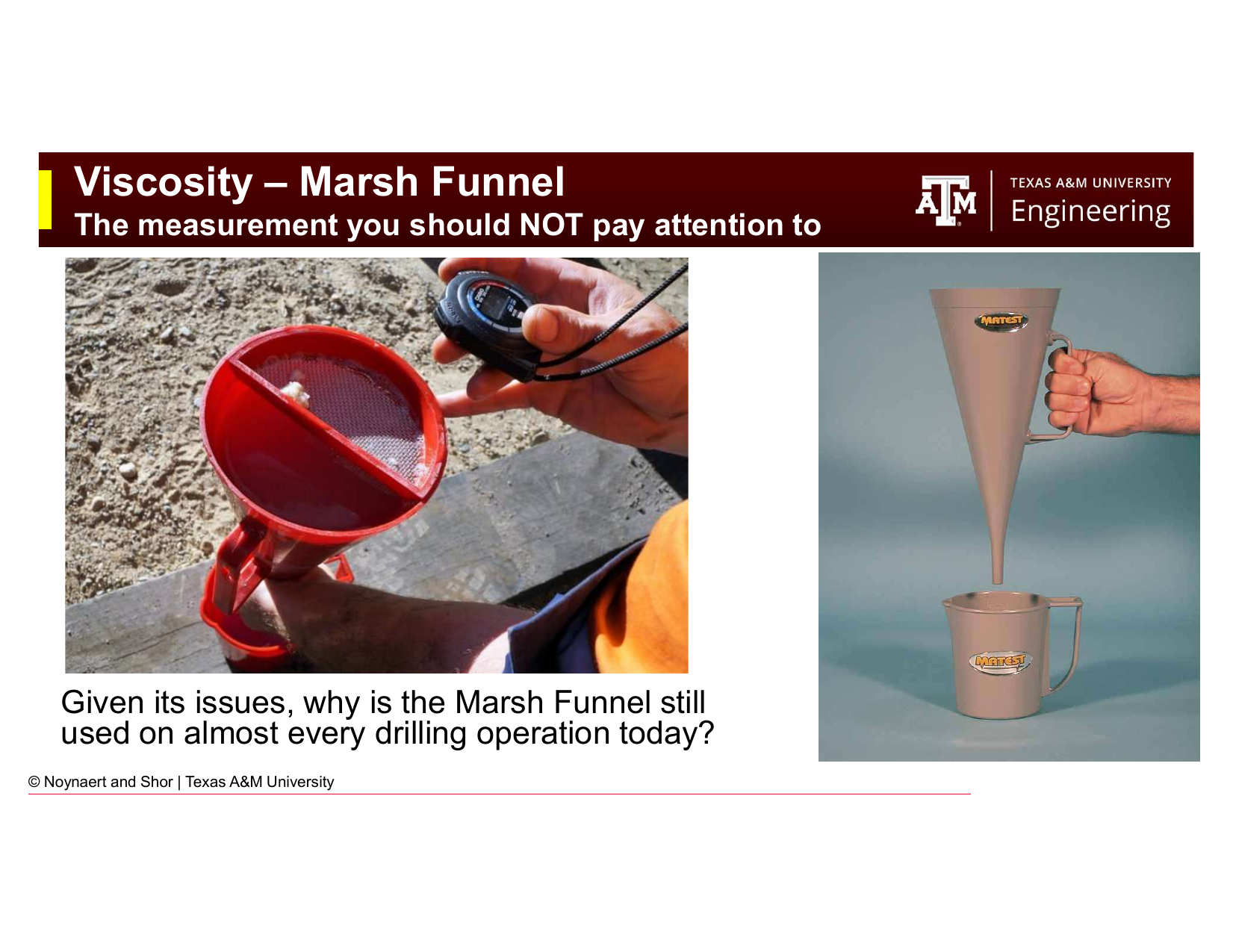
Fig. 51 The Marsh funnel — a simple, robust field viscosity indicator. One quart (946 mL) of mud is poured through the funnel and the time in seconds for one quart to drain is recorded.

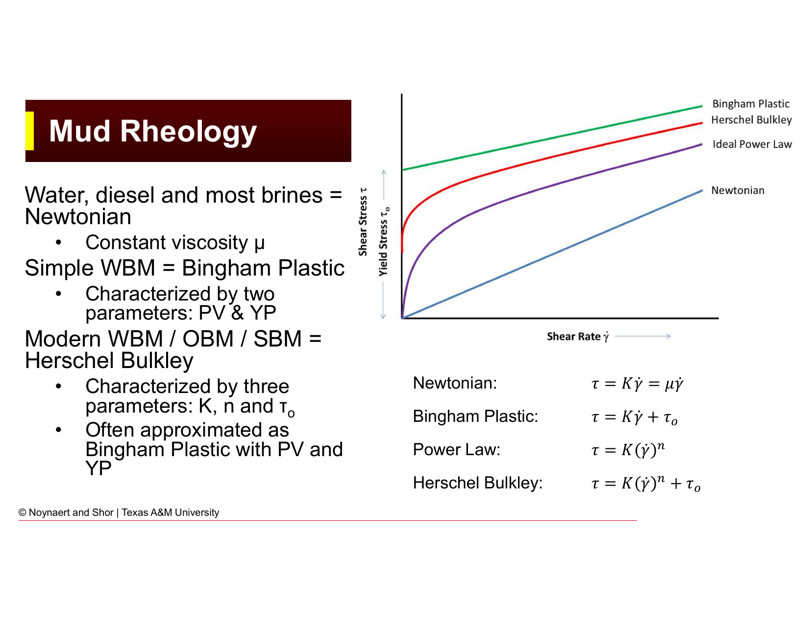
Fig. 52 Despite its significant limitations, the Marsh funnel remains in nearly universal use on drilling operations. Understanding why reveals something important about the nature of field measurements.

The Marsh funnel is a cone-shaped funnel through which a standard volume of mud (one quart or one liter, depending on the standard) is poured. The time in seconds for the fluid to drain through the orifice is recorded as the Marsh funnel viscosity.

The Marsh funnel does not measure viscosity at a fixed shear rate — as the funnel empties, the head pressure driving flow decreases, so the shear rate changes continuously during the measurement. This means the Marsh funnel result is a complex average of fluid behavior across a range of shear rates and is not directly comparable to a fundamental rheological parameter.

Reference values:

• Fresh water: ~26 sec/quart

• Bentonite mud: ~57 sec/quart (average shear rate ~18,000 s⁻¹)

• Xanthan-based mud: ~34 sec/quart (average shear rate ~42,000 s⁻¹)

Note that the xanthan mud, which is more viscous than water at low shear rates, flows faster than the bentonite mud through the Marsh funnel. This illustrates how misleading the Marsh funnel can be: because xanthan is highly shear-thinning (see Section 5.6), it has a much lower viscosity at the high shear rates in the funnel nozzle than bentonite does, and so it drains faster.

So why is the Marsh funnel still used on almost every drilling operation globally?

Despite these limitations, the Marsh funnel persists because it is:

• Fast — a complete reading takes under two minutes

• Cheap and robust — no moving parts, requires no calibration, impossible to break

• Sensitive to gross changes — large changes in mud condition (e.g., significant contamination, major viscosity swings) are immediately apparent

• Familiar to every driller — communication of a “funnel viscosity” is universal in the industry

The Marsh funnel is best understood as a simple, quick alarm system — not a precision rheological measurement. It reliably tells you if something has changed significantly; it does not tell you what that change is or why.

5.4.3 Automated Mud Rheology Systems

Newer systems are being deployed on drilling rigs which promise to automate the mud rheology measurement process. Some are simply automation wrapped around a simple Marsh Funnel or Fann 35 Viscometer. Newer systems consist of the following components:

• Automated In-line Sampling - either continuous sampling or automated interval sample collection from either the mud return line (low pressure) or on the standpipe (high pressure)

• Coriolis Flow Meter - to provide instantaneous density measurement

• Pipe Viscometer - a section of straight or curving pipe with known dimensions with pressure sensors to measure pressure drop. A high precision fluid pump is required to gather pressure drop readings at a range of shear rates

• Heater - required if temperature dependent property measurement is required

New Technology: Automated Mud Skid

Automated mud rheology measurement has been deployed in the field. Results from recent field trials can be found in the following SPE paper:

Gul, Sercan, et al. “[Automated Mud Check with an AI-Enhanced Automated Mud Skid: Results of a Long-Term Permian Field Trial.]{https://onepetro.org/SPEDC/proceedings-abstract/22DC/22DC/D031S022R002/482092}” SPE/IADC Drilling Conference and Exhibition. SPE, 2022.

---

5.5 Rheological Models

Fig. 53 The four primary rheological models used for drilling fluids, shown as shear stress vs. shear rate curves. Most real drilling muds are best described by the Herschel-Bulkley model, but are often approximated as Bingham Plastic for simplicity.

A rheological model is a mathematical equation that describes the relationship between shear stress and shear rate for a fluid. Different fluids follow different models, and selecting the appropriate model is necessary for accurate hydraulics calculations. In terms of complexity, a Newtonian Fluid exhibits linear behavior and is used to describe fresh water. A Bingham Plastic fluid is also linear, but requires an initial yield stress to begin flowing. An appropriate mental model for a Bingham Plastic fluid is toothpaste: toothpaste does not flow until squeezed. A Power Law fluid and a Herschel-Bulkley fluid add on a smooth transition from non-flowing to flowing behavior and are used to describe most viscous fluids.

5.5.1 Newtonian Fluids

\[\tau = \mu \dot{\gamma}\]

For a Newtonian fluid, shear stress is directly proportional to shear rate, with the proportionality constant being the viscosity \(\mu\). The viscosity is constant: it does not depend on how fast the fluid is being sheared.

Examples: Water, diesel, most brines, alcohols, benzene.

Fann meter: A Newtonian fluid produces dial readings that are directly proportional to rotor speed. Viscosity can be calculated from any single-speed reading:

\[\mu = \frac{300 \cdot \theta_N}{N}\]

where \(N\) is the rotor speed (rpm) and \(\theta_N\) is the dial reading at that speed.

5.5.2 Bingham Plastic Model

\[\tau = PV \cdot \dot{\gamma} + YP\]

The Bingham Plastic model describes fluids that require a minimum stress (the yield point, YP) before they begin to flow. Below the yield point, the fluid behaves as a rigid solid. Above it, the fluid flows with a constant slope (the plastic viscosity, PV).

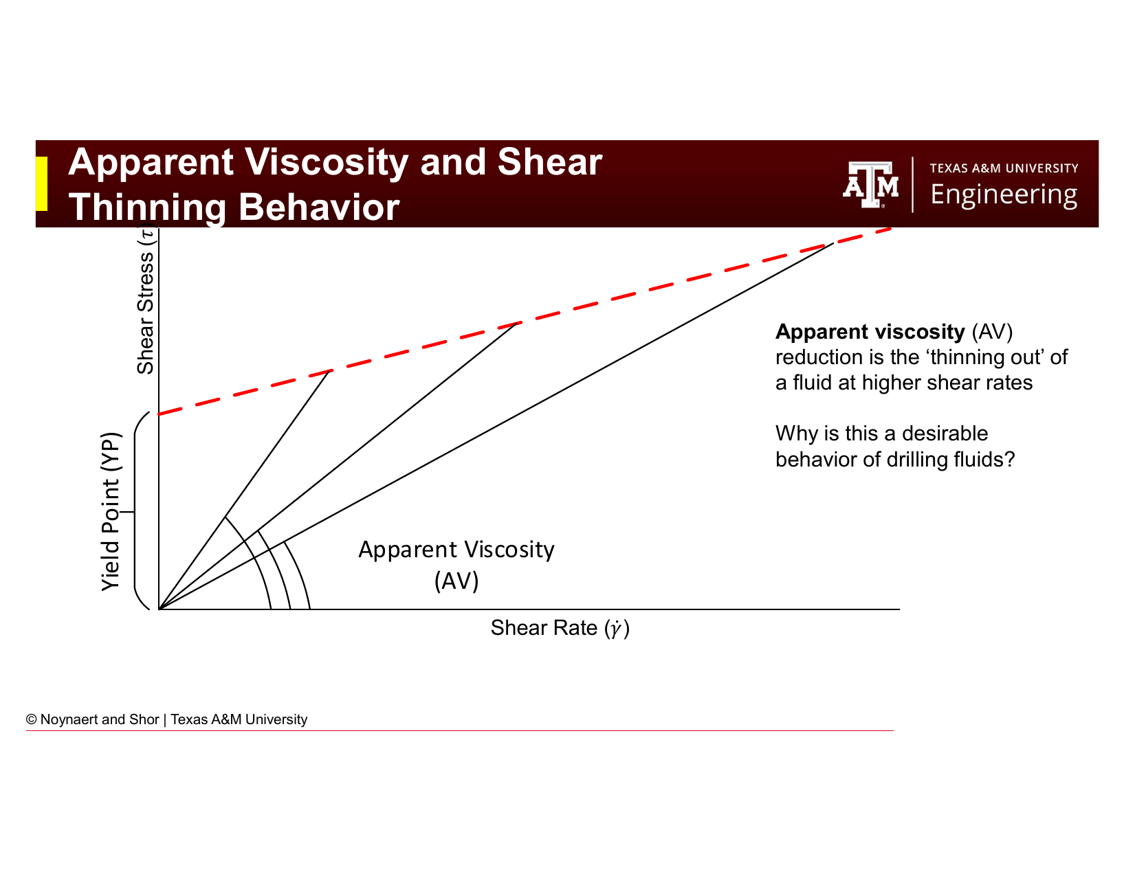
Fig. 54 Graphical illustration of the Bingham Plastic model. The plastic viscosity (PV) is the slope of the shear stress vs. shear rate line; the yield point (YP) is the y-intercept. In practice, PV and YP are calculated from the 600 and 300 rpm Fann readings.

Physical interpretation:

• Plastic Viscosity (PV) reflects the resistance to flow caused by mechanical friction between solid particles and between solids and the liquid phase. PV is primarily a function of mud solids content and their size distribution. High PV typically indicates excess solids.

• Yield Point (YP) reflects the attractive forces between particles in the mud at rest: the electrochemical and physical interactions that create a gel structure. YP governs the mud’s ability to suspend cuttings and weighting material. High YP is desirable for cuttings transport; excessively high YP increases pump pressures and surge/swab pressures.

Calculating PV and YP from Fann readings:

\[PV \text{ (cP)} = \theta_{600} - \theta_{300}\]

\[YP \text{ (lb/100 ft}^2) = \theta_{300} - PV = 2\theta_{300} - \theta_{600}\]

Typical values: For a well-designed WBM, PV is typically 10–20 cP and YP is 10–20 lb/100 ft².

5.5.3 Power Law Model

\[\tau = K \dot{\gamma}^n\]

The Power Law model captures the shear-thinning behavior of many drilling fluids, the tendency for apparent viscosity to decrease as shear rate increases, while maintaining a smooth derivative (slope). The two parameters are:

• \(K\) — the consistency index (a measure of overall fluid viscosity)

• \(n\) — the flow behavior index (dimensionless; \(n < 1\) for shear-thinning fluids, \(n = 1\) for Newtonian fluids)

The Power Law model does not include a yield stress — it predicts finite flow at any non-zero shear stress. This makes it a poor model at very low shear rates (annular conditions), where the yield stress behavior of real muds is important.

Calculating Power Law parameters from Fann readings:

\[n = 3.322 \log\left(\frac{\theta_{600}}{\theta_{300}}\right)\]

\[K = \frac{510 \cdot \theta_{300}}{511^n}\]

5.5.4 Herschel-Bulkley Model

\[\tau = K \dot{\gamma}^n + \tau_0\]

The Herschel-Bulkley (HB) model combines the yield stress of the Bingham Plastic with the shear-thinning behavior of the Power Law. It is the most physically accurate model for modern drilling fluids (WBMs, OBMs, SBMs) and requires three parameters: \(K\), \(n\), and \(\tau_0\) (yield stress).

Calculating HB parameters from 3, 6, 300, and 600 rpm Fann readings:

\[\tau_0 = 2\theta_3 - \theta_6\]

\[n = 3.322 \log\left(\frac{\theta_{600} - \tau_0}{\theta_{300} - \tau_0}\right)\]

\[K = \frac{510(\theta_{300} - \tau_0)}{511^n}\]

The HB model is the most computationally demanding of the four, which historically led to widespread use of the simpler Bingham Plastic approximation. Modern drilling software implements HB routinely.

5.5.5 Why Do Drillers Still Use the Bingham Plastic Model?

Fig. 55 The Bingham Plastic model significantly overestimates shear stress (and hence viscosity) at low shear rates compared to actual fluid behavior. Yet it remains in common use on mud reports and in field operations. Understanding why reveals important practical reasoning.

The Bingham Plastic model is known to overestimate fluid viscosity at low shear rates: it predicts that the fluid resists flow much more strongly in the slowly-flowing annulus than it actually does. Despite this, it remains on virtually every mud report and is still discussed as a primary model in the field. Why?

• Two-parameter simplicity. PV and YP can be calculated from any two Fann readings (600 and 300 rpm). Every mud engineer and driller can do this quickly at the rig site.

• Conservative design. Because the Bingham Plastic overestimates viscosity at low shear rates, hydraulics calculations using it tend to overestimate annular pressure losses and underestimate cuttings transport efficiency. For well control calculations, conservative estimates of equivalent circulating density (ECD) are safer than optimistic ones.

• Industry familiarity. PV and YP are universally understood. Communication across companies, engineers, and contractors is frictionless when everyone uses the same model.

• It works well enough at high shear rates. The pipe flow and bit conditions involve high shear rates where the Bingham Plastic and HB models converge. The overestimation error is most severe only at the low shear rates of the annulus.

The practical takeaway: use HB or Power Law for rigorous hydraulics design; use Bingham Plastic for quick field estimates and daily mud reporting. The Newtonian Fluid model should only be used if freshwater is being used as the drilling fluid.

---

5.6 Apparent Viscosity and Shear Thinning

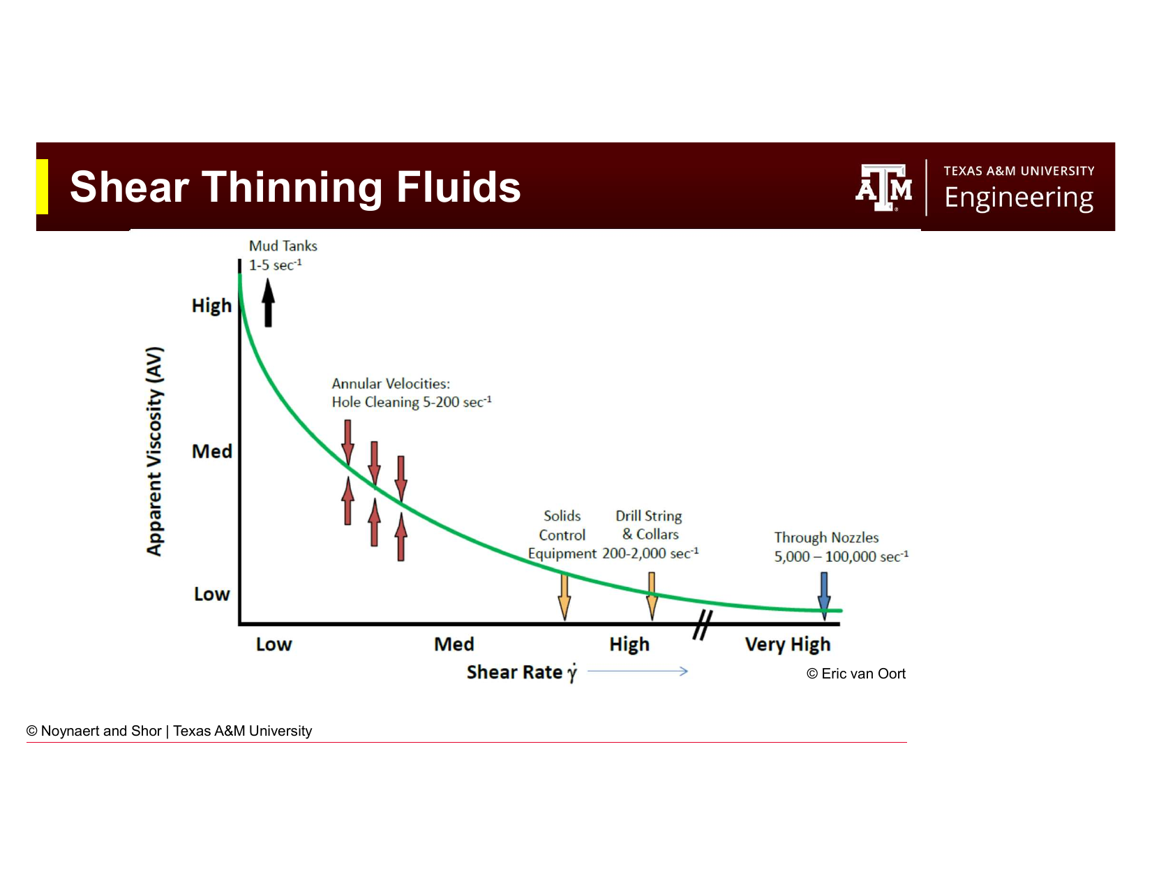
Fig. 56 Apparent viscosity as a function of shear rate for a shear-thinning (pseudoplastic) drilling fluid. At high shear rates (near the bit), the mud flows easily; at low shear rates (in the annulus), it is much more viscous and better able to carry cuttings.

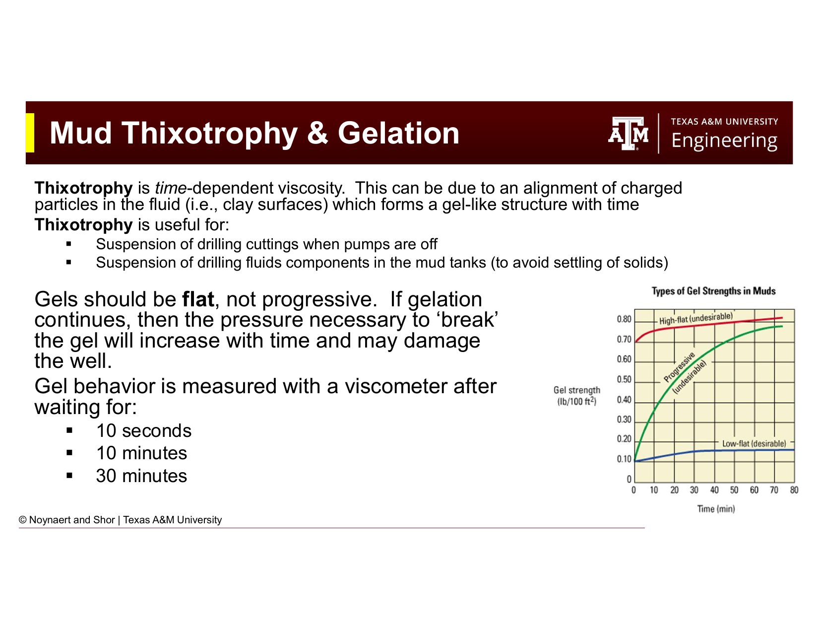
Fig. 57 Shear-thinning behavior demonstrated in drilling fluids. When the fluid experiences high shear (near the bit, through the nozzles), it thins dramatically; when it enters the slower-moving annulus, its viscosity recovers.

The apparent viscosity at a given shear rate is the ratio of shear stress to shear rate at that point:

\[\mu_{app} = \frac{\tau}{\dot{\gamma}}\]

For a Newtonian fluid, apparent viscosity is constant. For a shear-thinning (pseudoplastic) fluid, apparent viscosity decreases as shear rate increases — the fluid “thins out” under high shear and “thickens” when shear is reduced.

This behavior is highly desirable in drilling fluids because the flow conditions in different parts of the circulating system span an enormous range of shear rates:

Location	Approximate Shear Rate	Desired Viscosity
Bit nozzles	10,000–100,000 s⁻¹	Low (minimize pump pressure)
Drill pipe interior	500–1,500 s⁻¹	Moderate
Annulus	20–200 s⁻¹	High (carry cuttings)
Mud tank at rest	< 1 s⁻¹	Very high (suspend solids)

A shear-thinning mud naturally provides low viscosity where high flow speeds are needed (reducing pump pressure requirements and preventing hydraulic fracturing of the formation) and high viscosity where slow flow requires good cuttings suspension.

---

5.7 Thixotropy and Gel Strength

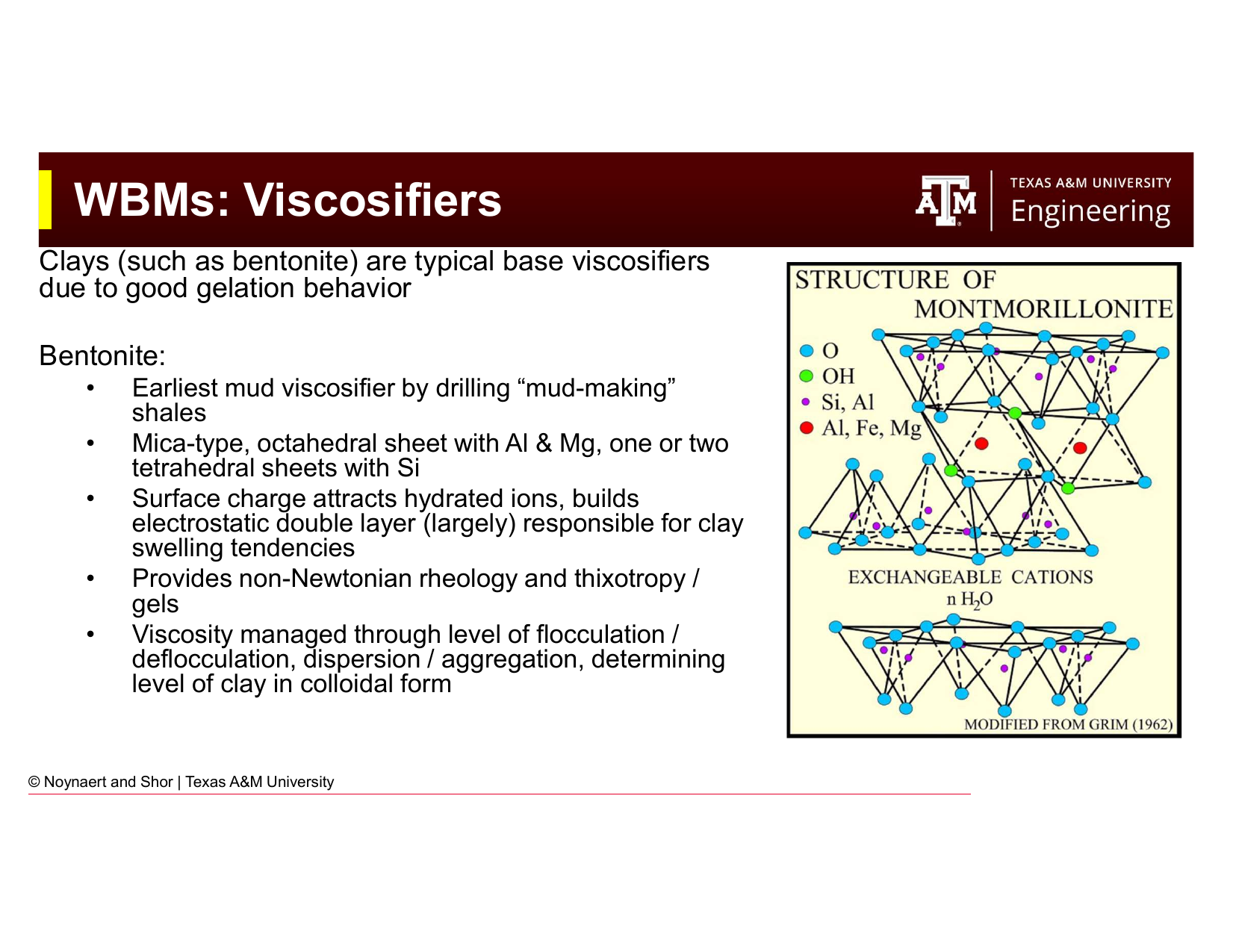
Fig. 58 Thixotropic vs. time-independent viscosity behavior. A thixotropic fluid’s viscosity increases with rest time as a gel structure develops. Ideal drilling fluid gels are “flat” — they build quickly to a limiting value and do not continue strengthening indefinitely.

Thixotropy is time-dependent viscosity: a fluid that becomes more viscous (gels) when at rest and returns to lower viscosity when sheared again. In drilling muds, thixotropy arises primarily from the alignment and association of charged clay platelets into a card-house gel structure when flow ceases.

5.7.1 Why Gel Strength Matters

Beneficial effects:

• When circulation is stopped (e.g., for a pipe connection), the gel structure holds drill cuttings in suspension in the annulus. Without gel strength, cuttings would settle to the bottom of the hole and pack around the bottom hole assembly and drillbit, potentially causing stuck pipe.

• The same gel structure keeps weighting materials (barite) suspended in the mud pits, preventing the dense solids from settling out and creating a non-uniform mud density.

Detrimental effects:

• When circulation is restarted after a long static period, the gel must be broken before the mud will flow. The pressure required to break the gel, the gel-breaking surge pressure, must not exceed the fracture gradient, or the formation will fracture and lead to lost circulation. Excessively strong gels after long shutdowns are a significant well control and wellbore stability concern.

• Progressive gels (ones that continue to strengthen with time) are particularly dangerous. If the gel strength doubles every hour, a 12-hour shutdown on a HPHT well can produce a gel so strong that restart may be impossible without fracturing the formation.

5.7.2 Ideal Gel Behavior: Flat Gels

The ideal gel is flat: it builds quickly to a moderate strength (good for cuttings suspension) and then does not increase significantly with time. The 10-second, 10-minute, and 30-minute gel strengths should be approximately equal, or the 10-minute gel should only be modestly higher than the 10-second gel.

Gel strength measurements (lb/100 ft²):

• After 10 seconds of rest

• After 10 minutes of rest

• After 30 minutes of rest

A mud with gels of 8/10/11 lb/100 ft² (10s/10min/30min) has flat, desirable gel behavior. A mud with gels of 4/16/45 lb/100 ft² has a progressive gel — a serious problem requiring treatment.

Key Term: Gel Strength

Gel strength is the maximum shear stress (measured in lb/100 ft²) required to initiate flow in a mud that has been at rest for a specified time period. It is measured with a Fann viscometer at 3 rpm after rest periods of 10 seconds, 10 minutes, and 30 minutes. Ideal muds have flat gel profiles (gel strength does not increase significantly with rest time).

---

5.8 Viscosifiers

5.8.1 Bentonite (Sodium Montmorillonite)

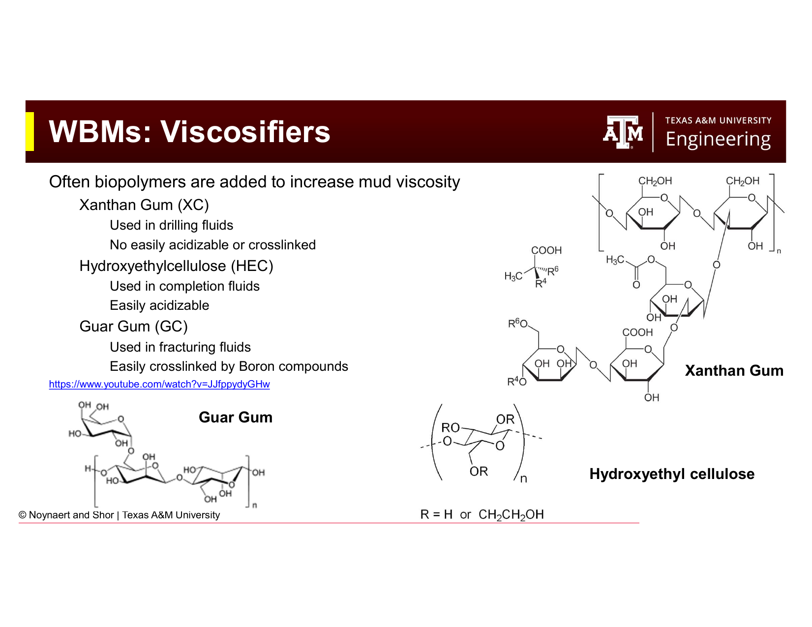
Fig. 59 The structure and mechanism of bentonite as a mud viscosifier. The charged clay platelets attract water molecules and form an electrostatic double layer that drives swelling and contributes to the gel structure of the mud.

Bentonite is the oldest and most widely used WBM viscosifier. It is a clay mineral (sodium montmorillonite) with a sheet-like crystal structure. Key characteristics:

• Surface charge — The clay platelet surfaces carry a net negative charge, while the platelet edges carry a positive charge. This creates an electrostatic double layer (EDL) around each particle.

• Hydration and swelling — The negative surface charge attracts a shell of hydrated cations (Na⁺, K⁺, Ca²⁺) and water molecules, causing the clay to swell. Sodium bentonite (Wyoming bentonite) swells up to 20 times its dry volume in fresh water, the most effective natural viscosifier.

• Gel structure — At rest, the attractive edge-to-face electrostatic interactions between platelets cause them to form a three-dimensional “card-house” network, creating the gel structure that gives bentonite muds their thixotropy.

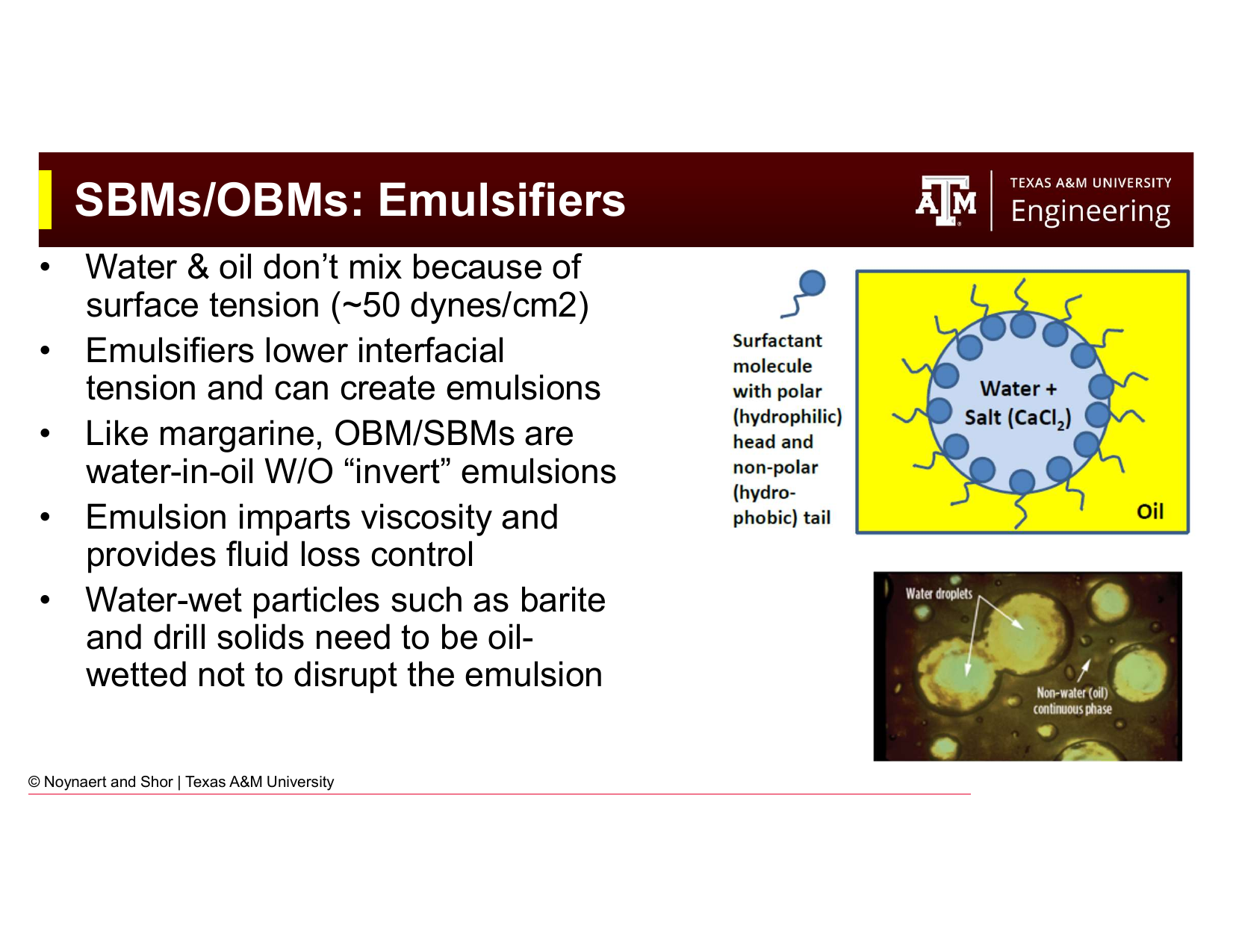
Fig. 60 Clay colloid behavior in different ionic environments. The degree of dispersion vs. aggregation, and flocculation vs. deflocculation, determines the viscosity and gel structure of a clay-based mud. Sodium montmorillonite in fresh water produces the most viscosity; calcium brines cause aggregation that reduces viscosity.

Clay behavior in mud is governed by the ionic environment:

• Dispersed and deflocculated (ideal for most operations) — clay platelets are well separated with no face-to-face stacking; provides smooth, controllable viscosity

• Aggregated — clay platelets associate face-to-face due to the influence of divalent ions (Ca²⁺, Mg²⁺); reduces viscosity and gel strength

• Flocculated — edge-to-face associations dominate; produces high viscosity and very progressive gels — often undesirable

Salt contamination (particularly calcium from cement or hard water) converts sodium montmorillonite to calcium montmorillonite, causing aggregation and dramatically reducing viscosity. This is one reason why WBMs are sensitive to cement contamination.

5.8.2 Biopolymer Viscosifiers

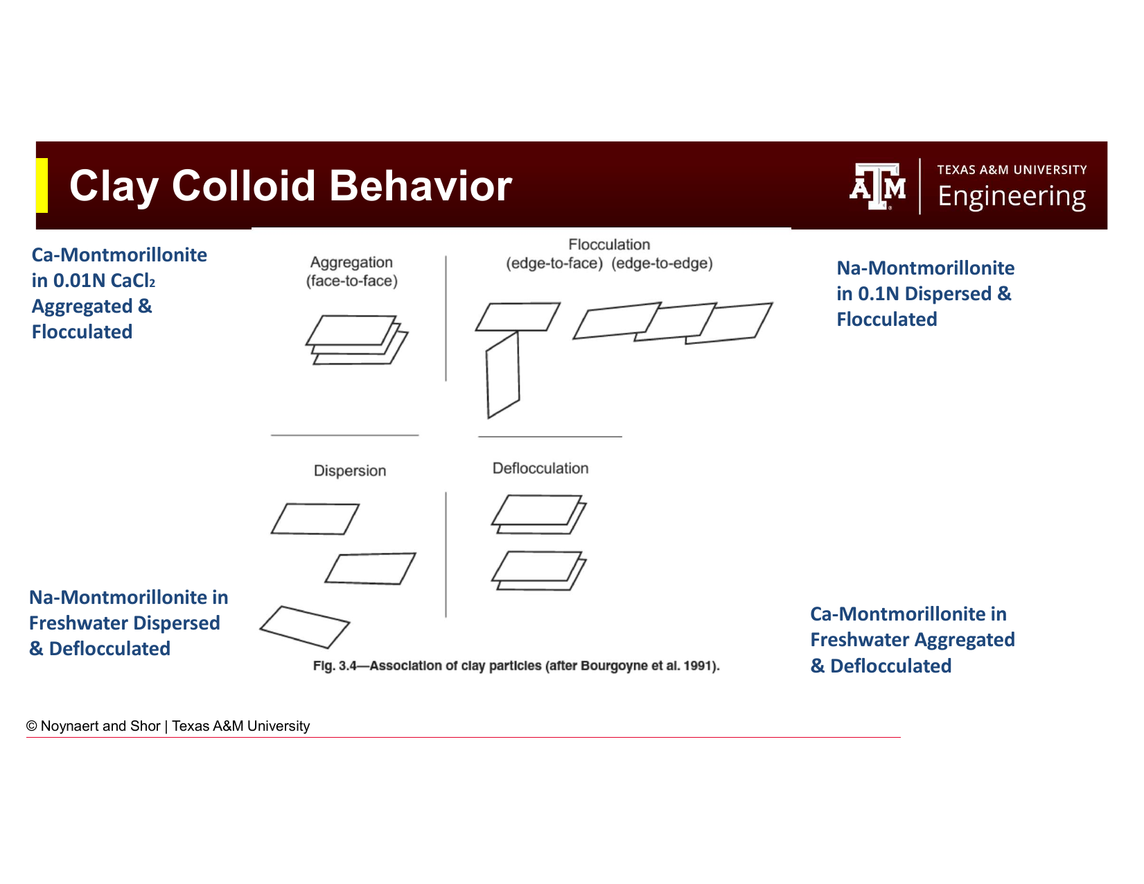
Fig. 61 The three primary biopolymer viscosifiers used in oilfield applications. Xanthan gum (XC) is the standard drilling fluid viscosifier; hydroxyethylcellulose (HEC) is preferred for completion fluids; guar gum is used in fracturing fluids.

Biopolymers are polysaccharide polymers produced by microbial fermentation. They provide viscosity through a different mechanism than clay — long polymer chains entangle and restrict relative motion of fluid layers. Key biopolymers in drilling:

Xanthan gum (XC polymer) — The standard polymer viscosifier for modern drilling fluids. Provides excellent shear-thinning behavior (viscosity at 3 rpm is much greater than viscosity at 600 rpm), good thermal stability to ~120°C, and is effective at very low concentrations (1–3 lb/bbl). XC cannot be easily crosslinked or acidized (which makes it persistent in the formation, a particular concern for reservoir sections).

Hydroxyethylcellulose (HEC) — Preferred in completion and workover fluids because it is easily degraded by acid, allowing cleanup of the filter cake after completion operations. Not used in drilling muds.

Guar gum — Used primarily in hydraulic fracturing fluids because it can be easily crosslinked with boron compounds to create high-viscosity gel systems at low pumping rates. Not commonly used in drilling.

5.8.3 OBM/SBM: Emulsifiers and Organophilic Clay

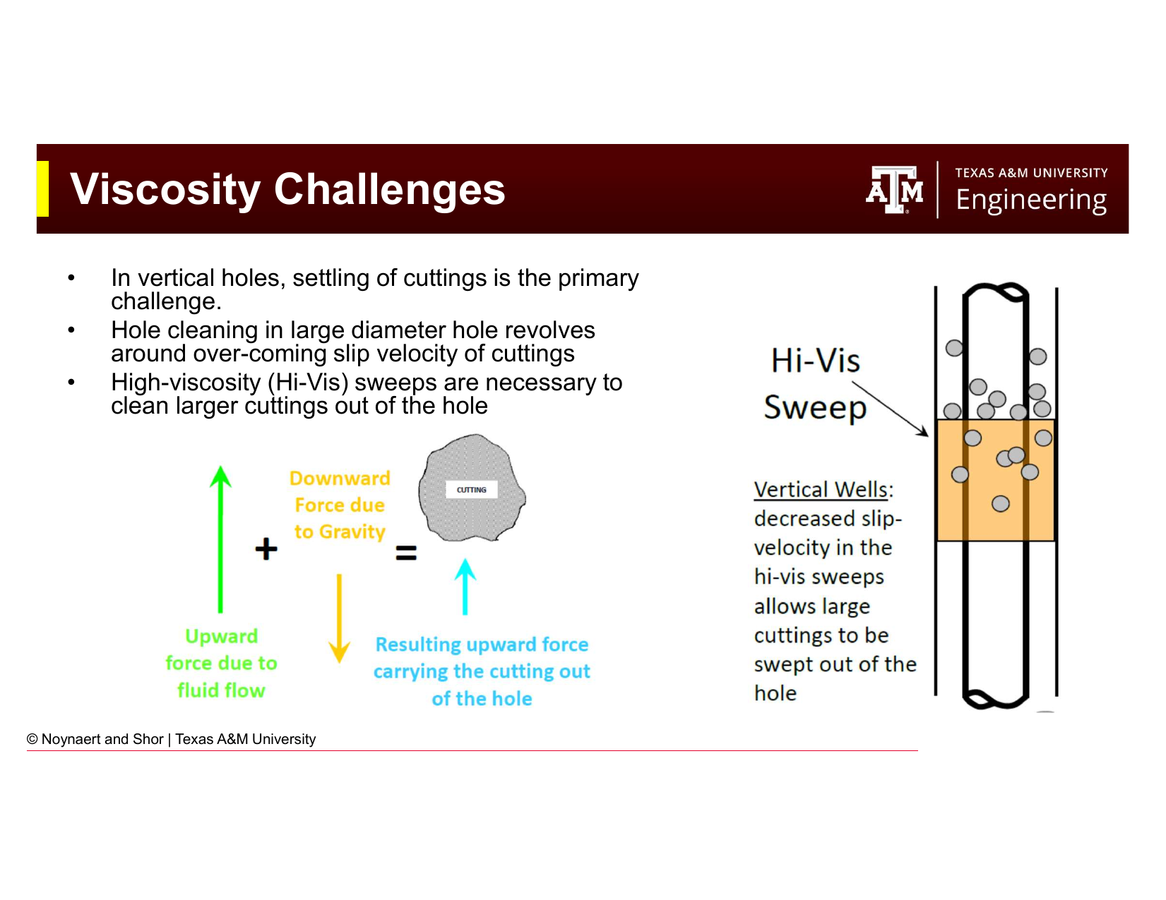
Fig. 62 The role of emulsifiers in OBM/SBM systems. Emulsifiers lower the interfacial tension between the oil and water phases, stabilizing the water-in-oil invert emulsion. They also convert water-wet particles (barite, drill solids) to oil-wet, preventing disruption of the emulsion.

In OBMs and SBMs, viscosity is provided by:

• Organophilic clay — clay that has been chemically treated with quaternary amines to make it oil-dispersible. Organophilic clay provides a gel structure in oil in the same way bentonite does in water.

• Organic polymers (dimer/trimer acids) — high-molecular-weight fatty acid derivatives that provide viscosity and fluid loss control in oil-continuous systems.

Emulsifiers are critical in OBM/SBM systems. They stabilize the water-in-oil emulsion by:

• Reducing interfacial tension between the oil and water phases from ~50 dynes/cm to near-zero

• Coating water droplets with a molecular film that prevents coalescence

• Converting water-wet particles (barite, drill solids) to oil-wet, keeping them dispersed in the oil phase

The emulsion stability of an OBM is measured with an electrical stability (ES) test — a high-voltage test that measures the breakdown voltage of the emulsion. High ES values indicate a robust emulsion; low ES values indicate emulsion instability and the risk of inversion (from water-in-oil to oil-in-water).

---

5.9 Viscosity Challenges in Hole Cleaning

5.9.1 Vertical Wells

In vertical wells, the primary challenge is overcoming the slip velocity of cuttings, the speed at which cuttings settle through the mud due to gravity. Larger and denser cuttings have higher slip velocities.

Strategies for effective vertical hole cleaning:

• Maximize annular velocity (higher pump rates)

• Increase mud viscosity (base viscosity and/or viscous sweeps)

• Control rate of penetration (ROP) — too fast generates more cuttings than the mud can carry

• Use high-viscosity (hi-vis) sweeps — periodic slugs of high-viscosity mud (typically 50–100 bbl) pumped to sweep accumulated cuttings beds from the hole

5.9.2 Horizontal Wells

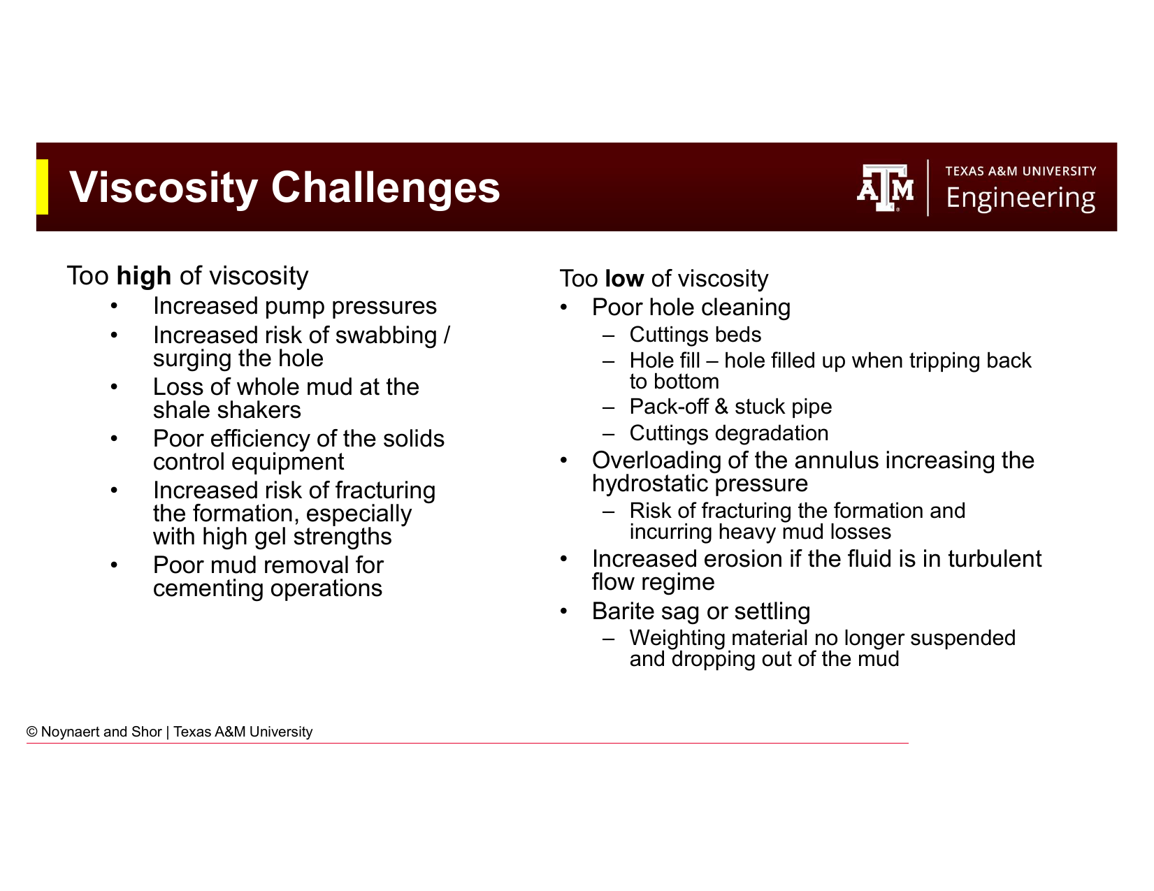
Fig. 63 Consequences of excessive viscosity (left) and insufficient viscosity (right). Mud viscosity must be optimized: too high and too low both cause serious operational problems.

In horizontal and highly deviated wells (inclination > 30°), the hole cleaning challenge is fundamentally different. Cuttings do not fall axially down the annulus — they fall radially and accumulate on the low side of the hole, forming cuttings beds. These beds can pack the annulus, cause stuck pipe, and increase torque and drag dramatically.

In horizontal wells:

• Viscosity has a much smaller effect on hole cleaning than in vertical wells. Once a cutting falls onto the low side of the annulus, the viscous drag from the mud flowing overhead has little ability to re-entrain it.

• Pump rate (annular velocity) and pipe rotation are the dominant factors. High flow rate turbulence and mechanical agitation from pipe rotation both help disturb and re-suspend cuttings beds.

• Equivalent circulating density (ECD) must be carefully managed: high pump rates increase ECD and risk lost circulation.

5.9.3 Consequences of Improper Viscosity

Too High Viscosity	Too Low Viscosity
Elevated pump and standpipe pressures	Poor hole cleaning — cuttings beds in deviated sections
Increased surge/swab pressures during tripping	Hole fill when tripping back to bottom
Lost mud at the shale shakers (mud too viscous to screen)	Pack-off and stuck pipe
Inefficient solids control equipment	Cuttings degradation (small particles harder to remove)
Risk of fracturing weak formations with high gel strengths	Overloaded annulus → increased ECD → lost circulation
Poor cement removal during cementing	Barite sag (weighting material settles out)

---

5.10 Fluid Loss Control

Fluid loss measurement and the physics of filter cake formation were introduced in Chapter 4. This section focuses on the measurement methods.

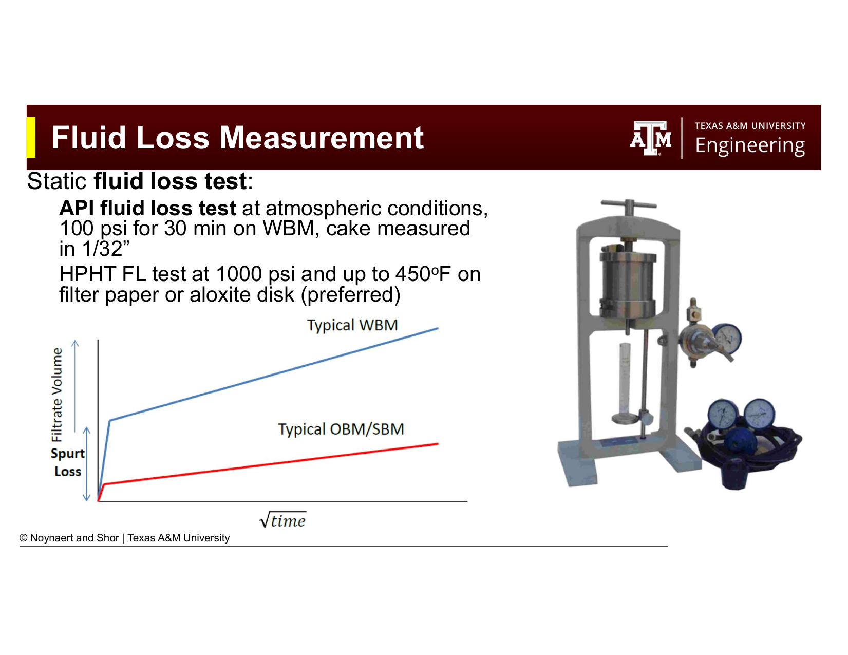
Fig. 64 The API fluid loss cell. The mud sample is loaded into the cell, 100 psi of pressure is applied across a standard filter paper, and the volume of filtrate collected in 30 minutes (in mL) is reported as the API fluid loss.

Standard API fluid loss test (LPLT — low pressure, low temperature):

• Pressure: 100 psi across a 90 mm diameter filter paper

• Temperature: ambient (typically 77°F / 25°C)

• Duration: 30 minutes

• Report: total filtrate volume in mL; filter cake thickness measured in 1/32 inch increments

HPHT fluid loss test (high pressure, high temperature):

• Pressure: 500 psi (differential)

• Temperature: up to 450°F (232°C); more commonly tested at 300–350°F for typical deep wells

• Filter medium: filter paper or ceramic aloxite disk (preferred for stability at high temperature)

• Required for deep, hot wells where API test conditions are unrepresentative

Typical API fluid loss targets:

• Standard WBM: ≤ 10–15 mL/30 min

• Low fluid loss WBM (e.g., for a deviated hole with stuck pipe risk): ≤ 5–8 mL/30 min

• OBM/SBM: ≤ 2–4 mL/30 min at 300°F (OBMs and SBMs have inherently better fluid loss control due to the emulsion structure)

---

5.11 Chemical Analysis

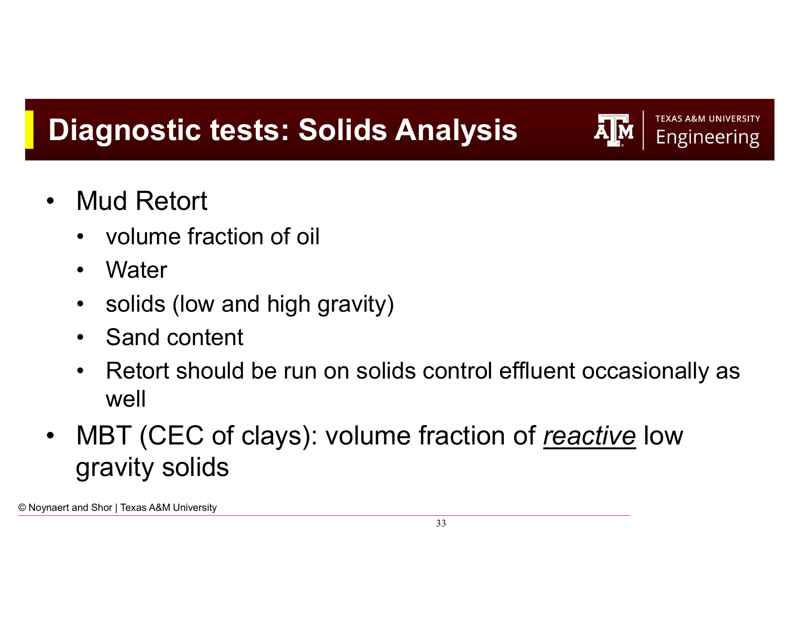
Fig. 65 Chemical analyses performed as part of a standard mud check: pH, chloride content, hardness, and alkalinity. These tests identify contamination and guide chemical treatment of the mud system.

Chemical analysis of the aqueous phase identifies contamination and tracks the chemical health of the mud system. Standard tests include:

pH — Measured with a pH meter or pH paper. Most WBMs are maintained at pH 9–11 (alkaline) to:

• Suppress corrosion of steel equipment

• Maintain effectiveness of pH-sensitive additives (many polymers and thinners work within specific pH windows)

• Inhibit bacterial degradation of organic additives

• Provide calcium contamination indication (high calcium drives pH down)

Chloride content — Measured by titration with silver nitrate. Tracks the salt content of the mud. Unexpectedly high chlorides may indicate salt formation drilling (halite dissolution) or saltwater influx from a formation.

Hardness (calcium and magnesium ions) — Measured by EDTA titration. Calcium (Ca²⁺) and magnesium (Mg²⁺) ions flocculate bentonite, increase fluid loss, and reduce the effectiveness of many additives. Hardness is a key indicator of cement contamination (from casing cement jobs) and formation water influx.

Alkalinity (P₁, P_m, M_m, M_f) — A series of titrations that quantify the concentrations of hydroxyl (OH⁻), bicarbonate (HCO₃⁻), and carbonate (CO₃²⁻) ions in the mud and mud filtrate. Alkalinity tests are used to:

• Confirm that sufficient lime is present in the system (as a contamination buffer)

• Detect CO₂ contamination (which forms carbonates and bicarbonates)

• Diagnose cement contamination (high alkalinity and calcium)

---

5.12 Solids Analysis

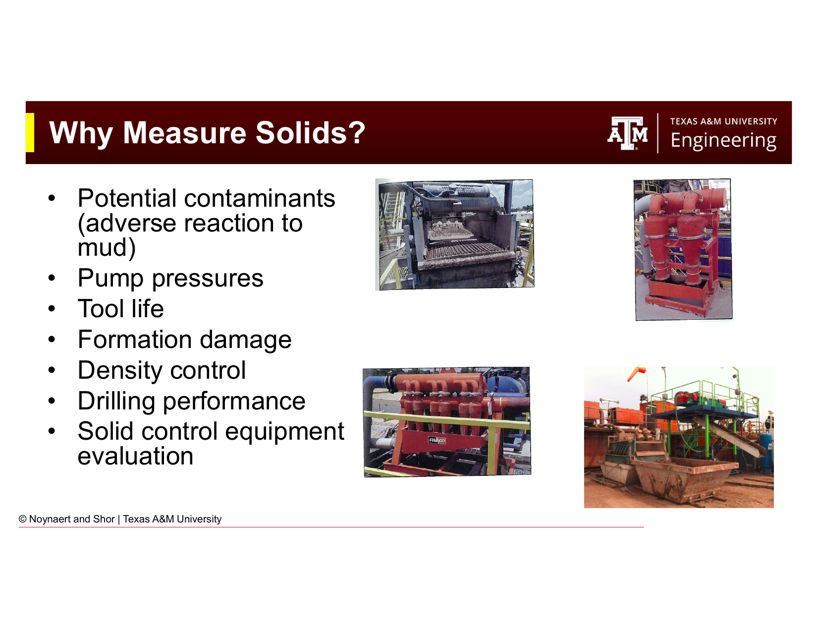
Fig. 66 Solids analysis tools: the mud retort (left) quantifies the volume fractions of oil, water, and solids; the methylene blue test (MBT, right) measures the cation exchange capacity of the clays to quantify reactive low-gravity solids.

Fig. 67 Why measuring solids matters. Solids content affects virtually every important mud property and operational metric: pump pressures, tool life, formation damage, density control, and drilling performance.

5.12.1 Mud Retort

The mud retort is the primary tool for solids analysis. A fixed volume of mud is heated in the retort apparatus to evaporate and condense all liquids. The condensate separates into oil and water layers, which are measured directly. Solids content (by volume) is calculated from the difference:

\[f_{solids} = 1 - f_{water} - f_{oil}\]

The retort gives total solids content but does not distinguish between different types of solids. To separate solids by specific gravity:

• High-gravity solids (HGS, SG ≥ 2.6): Barite (SG 4.2), hematite (SG 5.1), sand (SG 2.65). Added intentionally as weighting agents (except sand, which is a contaminant from the formation).

• Low-gravity solids (LGS, SG < 2.6): Drill solids (SG ≈ 2.6), clays (SG ≈ 2.4–2.6). Undesirable except for the intentionally added bentonite.

High LGS content degrades virtually every mud property: increases viscosity and gel strengths, reduces fluid loss control, reduces drilling performance, accelerates bit and pump wear, and makes density control difficult.

5.12.2 Sand Content

The sand content test uses a 200-mesh sieve to determine the volume fraction of coarse solids (> 74 µm). High sand content indicates:

• Inadequate solids control equipment performance

• Drilling of coarse-grained formations

• Poor sand screen management

High sand content accelerates erosive wear on pump liners, impellers, drill bits, and MWD tools.

5.12.3 Methylene Blue Test (MBT) — Cation Exchange Capacity

The methylene blue test (MBT) measures the cation exchange capacity (CEC) of the clays in a mud — essentially, how much bentonite (or other reactive clay) is present. Methylene blue dye binds to clay surface sites; the volume of dye solution required to fully saturate all clay sites is proportional to the total reactive clay content.

MBT is important because:

• Only the clay fraction of low-gravity solids contributes to viscosity and gel strength. Inert drill solids (quartz, feldspar) do not.

• Knowing the CEC allows the engineer to distinguish between a mud with high viscosity due to excess clay (treat with thinner/dilute) and one with high viscosity due to excess inert drill solids (dilute and improve solids control).

---

5.13 Contaminants

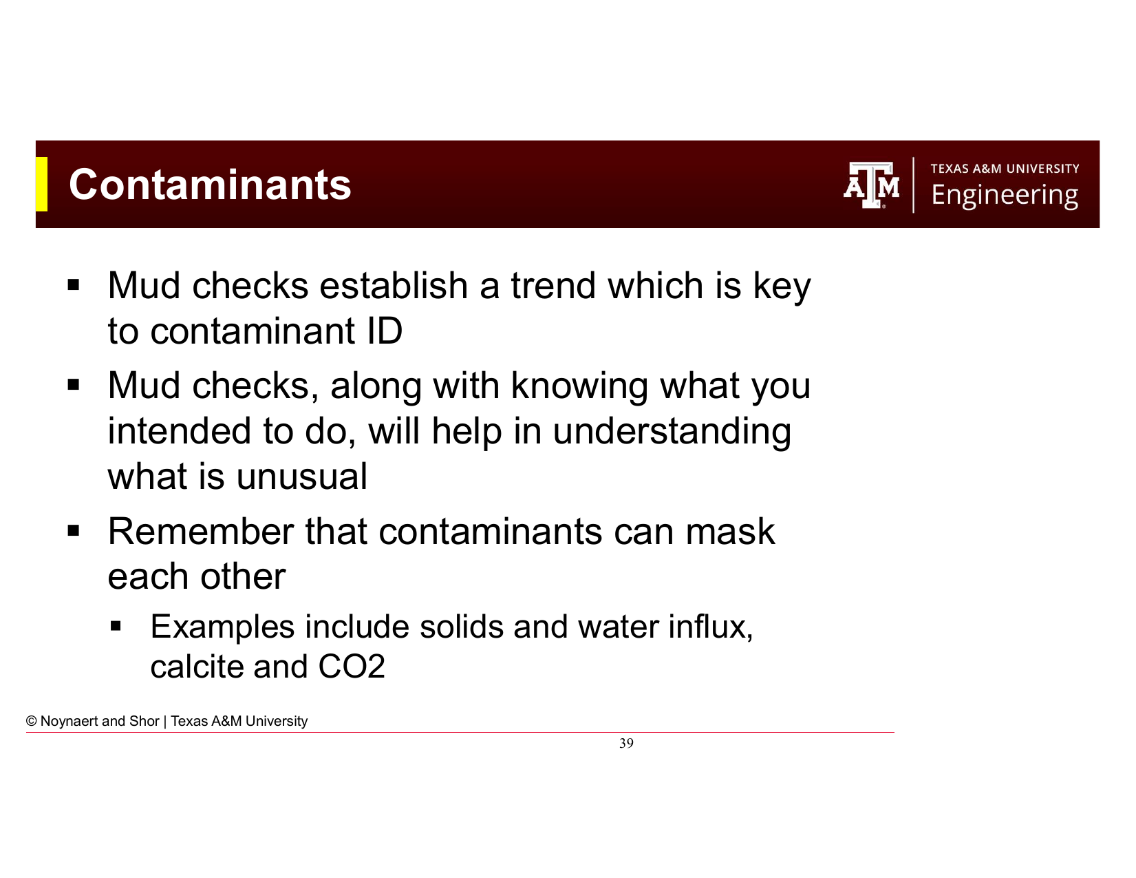
Fig. 68 Common drilling fluid contaminants, their sources, and their effects on mud properties. Regular mud checks establish the trend needed to identify contamination early.

Contaminants are materials that enter the mud from unintended sources and degrade its properties. Common contaminants and their sources include:

Salt (NaCl) — Source: halite or salt beds drilled through, saltwater formation influx. Effect: flocculates bentonite, reduces viscosity control, reduces effectiveness of many additives. Detection: chloride titration.

Calcium (Ca²⁺) — Source: cement (during casing operations), calcium-bearing formations (anhydrite, gypsum), hard supply water. Effect: flocculates bentonite dramatically, increases fluid loss, decreases pH, reduces polymer effectiveness. Detection: hardness titration. Treatment: addition of soda ash (Na₂CO₃) to precipitate calcium as calcium carbonate.

Carbon dioxide (CO₂) — Source: formations containing CO₂ gas, thermal degradation of organic additives. Effect: forms carbonates and bicarbonates that flocculate clays and increase fluid loss. Detection: alkalinity tests showing carbonate/bicarbonate presence. Treatment: lime addition.

Hydrogen sulfide (H₂S) — Source: sour formations containing H₂S gas. Effect: extremely hazardous to personnel (toxic at < 100 ppm, lethal at > 500 ppm); also causes sulfide stress cracking of high-strength steel in the drill string and BHA. Detection: gas detectors, Dräger tubes. Requires specialized mud treatment (iron-based H₂S scavengers) and respiratory protection protocols.

Drill solids — Source: formation being drilled. Effect: increase viscosity and gel strength, degrade fluid loss control, increase pump pressures. Detection: retort, MBT. Treatment: dilution, solids control equipment (shale shakers, centrifuges, desanders, desilters).

Key principle: mud checks establish trend. A single high calcium reading might be a measurement error; three consecutive readings showing increasing calcium over 12 hours indicate systematic contamination, likely from a cement job that has not fully been circulated out. Contaminants can also mask each other: a calcium influx from a formation and a CO₂ influx occurring simultaneously may produce intermediate chemistry readings that are confusing if interpreted individually rather than as a combined contamination event.

---

Worked Examples

Example 5.1 — Calculating PV, YP, and Apparent Viscosity

Problem: A Fann 35 viscometer gives the following readings for a WBM:

Speed (rpm)	Dial Reading (\(\theta\))
600	52
300	33
200	26
100	18
6	5
3	4

Calculate: (a) Plastic viscosity (PV), (b) Yield point (YP), (c) Apparent viscosity at 600 rpm, (d) Whether this mud is more viscous at 300 rpm or 600 rpm, and what that tells you about the fluid.

Solution:

(a) Plastic Viscosity:

\[PV = \theta_{600} - \theta_{300} = 52 - 33 = \boxed{19 \text{ cP}}\]

(b) Yield Point:

\[YP = \theta_{300} - PV = 33 - 19 = \boxed{14 \text{ lb/100 ft}^2}\]

(c) Apparent Viscosity at 600 rpm:

The Fann meter conversion gives apparent viscosity in cP as:

\[\mu_{app} = \frac{\theta_N \times 300}{N}\]

At 600 rpm:

\[\mu_{app,600} = \frac{52 \times 300}{600} = \boxed{26 \text{ cP}}\]

At 300 rpm:

\[\mu_{app,300} = \frac{33 \times 300}{300} = \boxed{33 \text{ cP}}\]

(d) Interpretation:

The apparent viscosity at 300 rpm (33 cP) is higher than at 600 rpm (26 cP) — the fluid is more viscous at the lower shear rate. This is the definition of shear-thinning behavior: viscosity decreases as shear rate increases. This is desirable: the mud will have relatively low viscosity near the bit (high shear) and relatively high viscosity in the annulus (low shear), which aids cuttings transport without excessive pump pressure.

---

Example 5.2 — Power Law Model Parameters

Problem: Using the Fann readings from Example 5.1, calculate the Power Law parameters \(n\) and \(K\).

Solution:

Flow behavior index \(n\):

\[n = 3.322 \log\left(\frac{\theta_{600}}{\theta_{300}}\right) = 3.322 \log\left(\frac{52}{33}\right)\]

\[n = 3.322 \times \log(1.576) = 3.322 \times 0.1975 = \boxed{0.656}\]

Since \(n < 1\), the fluid is confirmed to be shear-thinning (consistent with the apparent viscosity analysis above). An \(n\) value of 0.656 indicates moderate shear-thinning behavior — typical for a WBM with polymer viscosifier.

Consistency index \(K\):

\[K = \frac{510 \times \theta_{300}}{511^n} = \frac{510 \times 33}{511^{0.656}}\]

\[511^{0.656} = e^{0.656 \ln 511} = e^{0.656 \times 6.236} = e^{4.091} = 59.8\]

\[K = \frac{16{,}830}{59.8} = \boxed{281 \text{ mPa·s}^n \text{ (or equivalent cP-s}^{n-1}\text{)}}\]

Interpretation: The Power Law model for this mud is \(\tau = 281 \cdot \dot{\gamma}^{0.656}\), where \(\tau\) is in mPa and \(\dot{\gamma}\) is in s⁻¹.

---

Example 5.3 — Gel Strength Interpretation

Problem: A mud engineer records the following gel strength progression over the course of a 10-hour drilling pause for a mechanical repair:

Rest time	Gel strength (lb/100 ft²)
10 seconds	6
10 minutes	9
30 minutes	14
2 hours (estimated)	22
10 hours (estimated)	50

The fracture gradient at the weakest open-hole interval is 13.5 ppg EMW, corresponding to a maximum safe bottomhole pressure of 8,775 psi at 12,500 ft TVD. The static mud weight is 12.0 ppg (hydrostatic = 7,800 psi).

(a) Is this gel behavior flat or progressive? What are the implications?

(b) When the pumps restart after the 10-hour pause, the gel-breaking surge pressure adds temporarily to the hydrostatic. If the gel breaking requires a pressure spike of 450 psi above hydrostatic, will the formation fracture?

(c) What would you recommend to the mud engineer?

Solution:

(a) The gel strengths of 6/9/14 lb/100 ft² at 10s/10min/30min already show a rising trend, and the extrapolated values (22 at 2 hours, 50 at 10 hours) indicate a progressive gel — it is continuing to strengthen with no sign of leveling off. This is undesirable. After a 10-hour pause, restarting circulation will require significant pump pressure to break the gel, with a substantial surge pressure spike. The longer the pause continues, the worse this becomes.

(b) Maximum safe bottomhole pressure: 8,775 psi

Hydrostatic pressure: 7,800 psi

Pressure with gel-breaking surge: \(7,800 + 450 = 8,250\) psi

Since \(8,250 < 8,775\) psi, the formation will not fracture with the 450 psi spike. However, the safety margin is only \(8,775 - 8,250 = 525\) psi — relatively thin. If the gel continues to build and the required gel-breaking pressure rises above 975 psi, fracturing becomes a risk.

(c) Recommendations:

1. Treat the mud to reduce gel progression — add a thinner/deflocculant (e.g., lignosulfonate or PHPA) to reduce the rate of gel buildup. The goal is to achieve flat gels.

2. Break the gel gradually at pump startup — bring the pumps up slowly, increasing rate incrementally rather than starting at full pump speed.

3. Monitor the well closely — watch for lost circulation returns, pit volume changes, and surface pressure response during pump restart.

4. Limit the duration of any future static periods if gel behavior cannot be improved.

---

Practice Problems

5.1 A Fann 35 viscometer gives the following readings for an OBM at 150°F:

Speed (rpm)	Dial Reading
600	68
300	46
6	8
3	6

Calculate: (a) Plastic viscosity (PV) and yield point (YP) (b) Apparent viscosity at 600 rpm and at 300 rpm (c) Power Law parameters \(n\) and \(K\) (d) Herschel-Bulkley yield stress \(\tau_0\)

Solution

(a)

\[PV = \theta_{600} - \theta_{300} = 68 - 46 = \mathbf{22 \text{ cP}}\]

\[YP = \theta_{300} - PV = 46 - 22 = \mathbf{24 \text{ lb/100 ft}^2}\]

(b)

\[\mu_{app,600} = \frac{68 \times 300}{600} = \mathbf{34 \text{ cP}}\]

\[\mu_{app,300} = \frac{46 \times 300}{300} = \mathbf{46 \text{ cP}}\]

The apparent viscosity at 300 rpm is higher than at 600 rpm — confirming shear-thinning behavior.

(c)

\[n = 3.322 \log\left(\frac{68}{46}\right) = 3.322 \times \log(1.478) = 3.322 \times 0.1697 = \mathbf{0.564}\]

\[511^{0.564} = e^{0.564 \times 6.236} = e^{3.517} = 33.7\]

\[K = \frac{510 \times 46}{33.7} = \frac{23{,}460}{33.7} = \mathbf{696 \text{ mPa·s}^n}\]

(d) Herschel-Bulkley \(\tau_0\):

\[\tau_0 = 2\theta_3 - \theta_6 = 2(6) - 8 = \mathbf{4 \text{ lb/100 ft}^2}\]

Note: the OBM has a small but non-zero yield stress (4 lb/100 ft²), which the Bingham Plastic model captures as a much larger YP (24 lb/100 ft²) — illustrating the overestimation at low shear rates described in Section 5.5.5.

5.2 A mud engineer collects the following data during a routine mud check on a WBM at 11,500 ft TVD:

• Density: 13.2 ppg

• pH: 7.5

• Chlorides: 28,000 mg/L (baseline from the previous check: 4,200 mg/L)

• Hardness (as CaCO₃): 620 mg/L (baseline: 80 mg/L)

• 10-second gel: 8 lb/100 ft²

• 30-minute gel: 9 lb/100 ft²

• API fluid loss: 22 mL (baseline: 8 mL)

(a) Identify the likely source of contamination and explain your reasoning. (b) What are the two most operationally significant consequences of this contamination? (c) What chemical treatment would you recommend to address the calcium contamination?

Solution

(a) Calcium contamination, most likely from a cement job.

Evidence:

• Hardness increased from 80 to 620 mg/L — a large increase in Ca²⁺ concentration

• Chlorides also increased (from 4,200 to 28,000 mg/L), which could indicate saltwater from a formation OR from the mixing water used for cement (some cements use seawater or brackish water)

• pH dropped from presumably ~10 (baseline WBM) to 7.5 — calcium from cement neutralizes hydroxyl ions and drives pH down

• Fluid loss jumped from 8 to 22 mL — calcium flocculates bentonite and degrades polymer additives, destroying the fluid loss control package

The combination of high calcium, low pH, and high fluid loss strongly suggests cement contamination from the casing shoe or a cement squeeze job nearby.

(b) Two most significant consequences:

1. Loss of fluid loss control (API FL = 22 mL vs 8 mL baseline): Excessive filtrate invasion risks differential sticking and reservoir damage. This needs immediate treatment.

2. Reduced wellbore stability / mud property degradation: High calcium destroys bentonite structure and polymer effectiveness, which can cause viscosity instability. If the mud is being used to stabilize a reactive shale interval, loss of inhibition could cause borehole enlargement.

(c) Treatment:

Add soda ash (sodium carbonate, Na₂CO₃) to precipitate the calcium as calcium carbonate (calcite):

\[\text{Na}_2\text{CO}_3 + \text{Ca}^{2+} \rightarrow \text{CaCO}_3 \downarrow + 2\text{Na}^+\]

This removes Ca²⁺ from solution. Following the soda ash treatment:

• Increase caustic soda (NaOH) to restore pH to 9.5–10

• Add additional viscosifier (bentonite or XC polymer) to restore viscosity

• Add fluid loss control agent (starch or CMC) to restore API fluid loss to specification

• Monitor the mud closely over the next few circulations to ensure properties stabilize

5.3 A mud engineer records the following retort analysis on an 11.0 ppg WBM:

• Water: 72% by volume

• Oil: 0% by volume

• Solids: 28% by volume

The MBT test indicates that 8% of the total mud volume consists of reactive low-gravity solids (bentonite and reactive clays). Assume all remaining solids are inert high-gravity solids (barite, SG = 4.2) and inert low-gravity solids (drill solids, SG = 2.6).

(a) What is the total low-gravity solids (LGS) fraction? (b) What fraction of the total solids is LGS? (c) Industry guidelines suggest LGS should not exceed 6% by volume for good drilling performance. Is this mud within spec? (d) What operational measure would you take to reduce the LGS content?

Solution

(a) Total solids = 28% by volume.

To find the split between LGS and HGS, use the density relationship. The average solids density:

\[\rho_{solids} = \frac{\rho_{mud} - f_w \rho_w}{f_{solids}}\]

Mud density: 11.0 ppg → SG = 11.0/8.34 = 1.319

\[\rho_{solids,avg} = \frac{1.319 - (0.72)(1.0)}{0.28} = \frac{0.599}{0.28} = 2.14 \text{ SG}\]

Using the two-component mixing model for LGS (SG = 2.6) and HGS (SG = 4.2):

Let \(f_{LGS}\) = LGS fraction of total solids volume. Then:

\[2.14 = 2.6 f_{LGS} + 4.2(1 - f_{LGS})\]

\[2.14 = 2.6 f_{LGS} + 4.2 - 4.2 f_{LGS}\]

\[2.14 - 4.2 = -1.6 f_{LGS}\]

\[f_{LGS} = \frac{-2.06}{-1.6} = 0.7875 \approx 0.79\]

LGS fraction of total mud volume: \(0.28 \times 0.79 = \mathbf{22.1\%}\)

(b) Fraction of total solids that is LGS: 79%

(c) LGS = 22.1% by volume >> 6% guideline. This mud is significantly out of specification — LGS is more than 3.5× the recommended maximum. This level of drill solids will cause dramatically elevated viscosity, increased pump pressures, accelerated equipment wear, and poor drilling performance.

(d) To reduce LGS:

• Dilute the mud system by adding clean base fluid (water + fresh bentonite + additives) to replace the high-LGS mud. Dilution is the most common and effective approach.

• Improve solids control equipment performance — ensure shale shakers are running with the finest possible screens, that centrifuges are operational and processing a sufficient volume, and that desanders/desilters are functioning correctly.

• Consider a partial dump and replace — if LGS has built up to this level, dilution alone may be uneconomic; discard a portion of the active system and replace with fresh mud.

5.4 A deepwater well is being drilled with an SBM at 16,500 ft TVD. The mud engineer suspects H₂S contamination from a sour zone being drilled. The gas detectors show 45 ppm H₂S in the return gas.

(a) At 45 ppm, is this level immediately dangerous to life (IDLH threshold is typically 100 ppm for H₂S)?
(b) List three operational safety measures the rig crew should immediately implement.
(c) Describe the chemical treatment added to the mud to scavenge H₂S, and explain how it works.

Solution

(a) At 45 ppm, H₂S is below the IDLH threshold of 100 ppm — not immediately dangerous to life at this level. However, 45 ppm is well above the OSHA permissible exposure limit (PEL) of 20 ppm and the immediately detectable odor threshold (~0.5 ppm). Workers on the rig floor and at the shale shakers would be at risk without respiratory protection. Personnel should not be working in the affected area without appropriate PPE (self-contained breathing apparatus or air-supplied respirators).

(b) Immediate operational safety measures:

1. Activate H₂S response plan — notify the company man, drill crew, and safety officer; muster all personnel to upwind muster stations

2. Issue and don personal H₂S monitors (badge-type and electronic) for all personnel in the hazardous zone; ensure air-supplied breathing apparatus is available and functional at all muster points

3. Increase the H₂S scavenger treatment rate in the mud system and verify the gas detection equipment is calibrated and alarming at appropriate setpoints (typically 10 ppm for alarm, 25 ppm for evacuation)

(c) H₂S scavengers for mud systems are typically iron-based compounds — most commonly iron oxide (hematite, Fe₂O₃) or iron carbonate-based products. The reaction:

\[\text{Fe}_2\text{O}_3 + 3\text{H}_2\text{S} \rightarrow \text{Fe}_2\text{S}_3 + 3\text{H}_2\text{O}\]

The iron oxide converts the dissolved H₂S into insoluble iron sulfide, removing the H₂S from the liquid phase and preventing it from flashing out of solution at the shale shakers (where the pressure drops to atmospheric). Zinc-based scavengers are also used but are increasingly restricted offshore due to toxicity. The scavenger must be maintained in excess of the H₂S concentration — typically added continuously at the suction pit as a routine treatment when drilling known sour zones.

5.5 Compare the Bingham Plastic and Herschel-Bulkley rheological models using the following Fann data from a modern SBM:

Speed (rpm)	600	300	6	3
Dial reading	74	50	7	5

(a) Calculate PV and YP (Bingham Plastic). (b) Calculate \(\tau_0\), \(n\), and \(K\) (Herschel-Bulkley). (c) Calculate the predicted shear stress at 3 rpm using both models and compare to the measured value. Which model is more accurate at low shear rates? (d) Why does this difference matter for drilling hydraulics calculations?

Solution

(a) Bingham Plastic:

\[PV = 74 - 50 = \mathbf{24 \text{ cP}}\]

\[YP = 50 - 24 = \mathbf{26 \text{ lb/100 ft}^2}\]

(b) Herschel-Bulkley:

\[\tau_0 = 2\theta_3 - \theta_6 = 2(5) - 7 = \mathbf{3 \text{ lb/100 ft}^2}\]

\[n = 3.322 \log\left(\frac{74 - 3}{50 - 3}\right) = 3.322 \log\left(\frac{71}{47}\right) = 3.322 \times \log(1.511) = 3.322 \times 0.1793 = \mathbf{0.596}\]

\[511^{0.596} = e^{0.596 \times 6.236} = e^{3.717} = 41.1\]

\[K = \frac{510(47)}{41.1} = \frac{23{,}970}{41.1} = \mathbf{583 \text{ mPa·s}^n}\]

(c) Predicted shear stress at 3 rpm (shear rate = 5.1 s⁻¹):

Bingham Plastic: \(\tau = PV \cdot \dot{\gamma} + YP\)

At 3 rpm: \(\tau = 24 \times (5.1/300) + 26 = 0.41 + 26 = \mathbf{26.4 \text{ lb/100 ft}^2}\)

(Note: using the Fann approximation, \(\tau_{BP,3rpm} \approx PV/100 + YP = 26.2\) lb/100 ft² — effectively the Bingham plastic predicts ~26 lb/100 ft² at 3 rpm)

Herschel-Bulkley: \(\tau = K \dot{\gamma}^n + \tau_0 = 583 \times (5.1)^{0.596} + 3\)

\((5.1)^{0.596} = e^{0.596 \ln 5.1} = e^{0.596 \times 1.629} = e^{0.971} = 2.64\)

\(\tau = 583 \times 2.64 / 300 + 3 \approx 5.13 + 3 = \mathbf{8.1 \text{ lb/100 ft}^2}\)

(using consistent units with the Fann factor)

Measured value at 3 rpm: 5 lb/100 ft²

The Herschel-Bulkley prediction (≈8 lb/100 ft²) is much closer to the measured value (5 lb/100 ft²) than the Bingham Plastic prediction (≈26 lb/100 ft²). The Bingham Plastic overestimates by 5× at low shear rates.

(d) This matters for annular hydraulics calculations. The low-shear region (3–100 rpm Fann readings) corresponds to the shear conditions in the annulus, particularly in large-diameter surface casing sections. If the Bingham Plastic model is used, annular pressure losses will be significantly overestimated, leading to conservative ECD predictions. In a well with a narrow drilling window (small margin between pore pressure and fracture gradient), this overestimation could lead to unnecessarily conservative mud weight decisions, or — in the opposite direction — the engineer might become complacent because “the model says we have 2 ppg margin” when the true margin is less. Using HB for design and BP for quick field communication is the appropriate engineering approach.

---

Summary

This chapter has covered the measurement and interpretation of drilling fluid properties:

• Regular mud monitoring establishes trends that allow problems to be caught and corrected before they become expensive. Mud checks are taken from the active pit (suction) for normal reporting, and from the return line to detect contamination or influx.

• Density is measured with the pressurized mud balance (field standard) or in-line Coriolis meters (continuous, but limited by gas sensitivity). The pressurized cap corrects for gas-cut mud errors.

• Viscosity is measured with the Fann VG/35 viscometer (the precision field instrument, providing measurements at six standard speeds) or the Marsh funnel (a rapid but imprecise indicator useful only for detecting gross changes).

• Four rheological models describe mud behavior: Newtonian (one parameter), Bingham Plastic (PV + YP, calculated from 600 and 300 rpm readings), Power Law (\(K\) and \(n\)), and Herschel-Bulkley (\(K\), \(n\), and \(\tau_0\)). The Bingham Plastic remains in wide use despite its known overestimation at low shear rates because it is fast, simple, and conservative.

• Shear-thinning behavior (decreasing apparent viscosity at higher shear rates) is desirable — it provides low viscosity near the bit and high viscosity in the annulus.

• Thixotropy and gel strength are essential for cuttings suspension during static periods. Gels should be flat (not progressive) to avoid excessive gel-breaking surge pressures on restart.

• Viscosifiers include bentonite (clay-based, provides both viscosity and thixotropy via electrostatic interactions) and biopolymers (especially xanthan gum, providing shear-thinning viscosity at low concentration). OBMs use organophilic clay and emulsifiers.

• Chemical analysis (pH, chlorides, hardness, alkalinity) and solids analysis (retort, sand content, MBT) together provide a complete picture of mud condition and identify contamination. Trending across multiple mud checks is more diagnostic than any single data point.

• Common contaminants include salt, calcium (from cement), CO₂, H₂S, and excess drill solids, each with characteristic effects on mud properties and specific treatments.

Chapter 6 covers the calculations used to design mud density, mix mud systems, and perform basic hydraulics calculations, applying the fluid properties characterized in this chapter.

---

References

Mitchell, R.F. and Miska, S.Z. (eds.), Fundamentals of Drilling Engineering, Society of Petroleum Engineers, 2011.

Al-Majed, A.A., Hossain, M.E., and Al-Majed, A., Fundamentals of Sustainable Drilling Engineering, John Wiley and Sons, 2015.

API RP 13B-1, Recommended Practice for Field Testing Water-based Drilling Fluids, American Petroleum Institute.

API RP 13B-2, Recommended Practice for Field Testing of Oil-based Drilling Fluids, American Petroleum Institute.

API RP 13D, Rheology and Hydraulics of Oil-well Drilling Fluids, American Petroleum Institute.