
Chapter 13 — Advanced Directional Drilling Topics#
Learning Objectives#
By the end of this chapter, you should be able to:
Compare the survey calculation methods used in industry (average angle, radius of curvature, constant build and turn, minimum curvature) and explain why minimum curvature is the standard.
Apply the minimum curvature method to a 3D survey interval: compute the dogleg angle, ratio factor, and position increments, and calculate dogleg severity from survey data.
Explain the physical origin of torque and drag and how hookload differs between pick-up, slack-off, and rotating-off-bottom operations.
State the assumptions of the soft-string model and write the Johancsik force balance for a drillstring element.
Carry out the Johancsik calculation procedure element by element from the bit to surface, computing tension and torque profiles for a deviated well.
Calibrate a friction factor from measured hookload data and use torque and drag analysis in well design and real-time monitoring.
Describe the limitations of the soft-string model, the motivation for stiff-string models, and the basic modes of drillstring vibration.
13.1 From Planning Tools to Engineering Models#
Chapter 12 developed the radius of curvature method for 2D well planning and introduced the minimum curvature method and torque and drag conceptually. This chapter completes both topics quantitatively.
The distinction matters in practice. A planned well is a smooth geometric idealization; a drilled well is known only through discrete survey stations measured every ~30–100 ft, with inclination and azimuth both changing between stations. Turning those discrete measurements into a 3D position — and into the contact forces that determine whether the string can be rotated, advanced, and pulled — requires the two models developed here.
13.2 Survey Calculation Methods#
Several methods exist for computing wellbore position from survey measurements (MD, inclination \(I\), azimuth \(Az\) at each station). They differ in what they assume the wellpath does between stations:
Average Angle Method (AAM): Inclination and azimuth are assumed constant and equal to the average of the two station values. Simple, and adequate for short intervals with small angle changes.
Radius of Curvature Method (RCM): Build rate and horizontal turn rate are assumed constant over the interval — the path is an arc in the vertical plane and an arc in the horizontal plane (Chapter 12, Section 12.2).
Constant Build and Turn Method (CBTM): Build rate and turn rate are constant over the trajectory.
Constant Curvature and Build Method (CCBM): The constant tool face method.
Minimum Curvature Method (MCM): The wellpath between stations is the shortest smooth arc joining the two measured direction vectors — a circular arc lying in the plane defined by the two vectors. This is the most widely used method in the petroleum industry, for both well trajectory planning and directional survey evaluation.
The minimum curvature method won industry-wide adoption because its single assumption — a circular arc turning in the plane of the two survey vectors — is the most defensible when nothing is known about the path between stations, and because it handles simultaneous inclination and azimuth change without special cases.
13.3 The Minimum Curvature Method#
13.3.1 The Dogleg Angle#
The total 3D angular change between two stations — the dogleg angle \(\beta\) — follows from the dot product of the two unit direction vectors:
with \(\beta\) in radians. Note the structure: for no azimuth change, \(\beta = I_2 - I_1\) (pure build); for no inclination change, the azimuth term alone contributes, scaled by \(\sin I_1 \sin I_2\) — azimuth changes matter more at high inclination.
Dogleg severity is the dogleg angle normalized per 100 ft:
13.3.2 The Ratio Factor#
The ratio factor corrects the chord-average direction for the curvature of the arc:
For a straight interval, \(RF \to 1\) as \(\beta \to 0\) (use \(RF = 1\) when \(\beta\) is very small to avoid division by zero). Even at a severe 10°/100 ft dogleg over a 100 ft interval, \(RF = 1.00254\) — the correction is small but is always applied in survey processing.
13.3.3 Position Increments#
With \(\beta\) and \(RF\) known, the position increments over the interval of length \(\Delta MD\) are:
Summing the increments station by station from the surface location gives the complete 3D wellpath.
13.3.4 Worked Example: A 3D Survey Interval#
Given: Two consecutive survey stations in a well that is building angle and turning:
Station |
MD (ft) |
Inclination |
Azimuth |
|---|---|---|---|
1 |
5,000 |
30° |
40° |
2 |
5,100 |
34° |
48° |
Find: The dogleg angle, DLS, ratio factor, and position increments.
Step 1 — Dogleg angle.
Step 2 — Dogleg severity.
Note that the inclination change alone is only 4°/100 ft — the azimuth change adds significantly to the total curvature at this inclination.
Step 3 — Ratio factor.
Step 4 — Position increments.
Over this 100 ft of measured depth, the well gains 84.8 ft of TVD and moves 37.9 ft north and 36.9 ft east. Repeating this calculation at every survey station builds the position log used for target steering and anti-collision analysis.
MCM in Practice
Every commercial survey processing package uses the minimum curvature method. The by-hand competency matters because the drilling engineer must be able to check the software: a transposed inclination, an azimuth referenced to the wrong north, or a misplaced decimal in a survey produces position errors that propagate to every station below — and the first line of defense is an engineer who can spot-check an interval by hand.
13.4 Torque and Drag: The Physical Picture#
13.4.1 Why Torque and Drag Exist#
In a perfectly vertical well, the drillstring hangs freely: the hookload equals the buoyed string weight, and surface torque equals bit torque. In any deviated well, the string must bend to follow the wellpath, and it lies against the borehole wall along inclined and curved sections. Every point of contact carries a normal force, and every normal force generates Coulomb friction opposing whatever motion the string makes:
Moving the string up (picking up): friction acts downward — hookload exceeds buoyed weight.
Moving the string down (slacking off): friction acts upward — hookload is less than buoyed weight.
Rotating the string: friction acts circumferentially — it consumes surface torque rather than axial force.
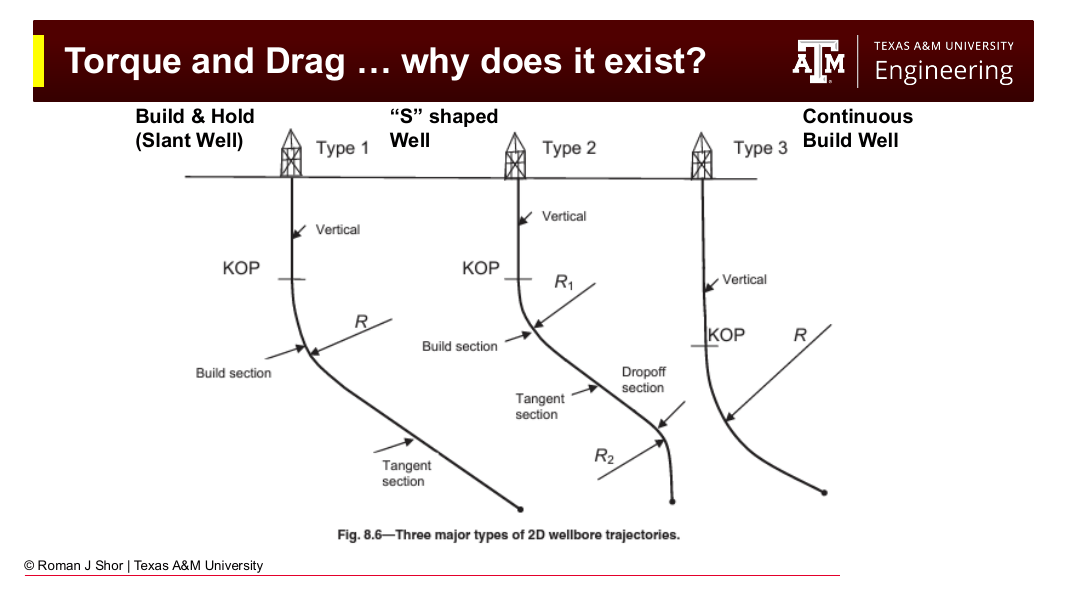
Fig. 177 The standard 2D wellbore profiles — build-and-hold (slant), S-shaped, and continuous build. Every departure from vertical creates wall contact, and every wall contact contributes to torque and drag.#
The difference between pick-up weight, rotating-off-bottom weight, and slack-off weight — measured routinely on every connection — is the field signature of drag, and (as Section 13.6 shows) the primary data used to calibrate torque and drag models.
13.4.2 Contact Force Sources#
Two mechanisms generate normal force on a drillstring element:
Gravity on inclined hole: An element of buoyed weight \(W\) at inclination \(\theta\) presses against the low side of the hole with force \(W \sin\theta\). This dominates in tangent and lateral sections.
Tension through curvature: A tensioned string pulled through a dogleg presses against the wall like a rope over a pulley. The normal force scales with the tension times the angular change — which is why doglegs high in the well, where tension is greatest, are so much more costly than the same dogleg near the bit.
The Johancsik model quantifies both.
13.5 The Johancsik Soft-String Model#
The industry-standard torque and drag model was published by Johancsik, Friesen, and Dawson in 1984 (Torque and Drag in Directional Wells — Prediction and Measurement, Journal of Petroleum Technology). Forty years later, it remains the default model in every commercial torque and drag package.
13.5.1 Assumptions#
The model treats the drillstring as a soft string — a heavy, flexible cable:
The string has weight but no bending stiffness: it conforms exactly to the wellbore trajectory.
Contact with the wellbore is continuous along each element (no discrete contact points at tool joints).
Friction is Coulomb friction: friction force = \(\mu \times\) normal force, with a single friction factor \(\mu\) (or one for cased hole and one for open hole).
The wellpath is known from the survey (processed by minimum curvature — the two halves of this chapter meet here).
13.5.2 The Element Force Balance#
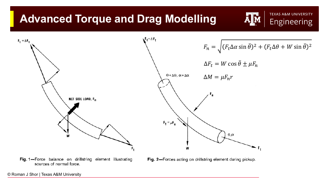
Fig. 178 The Johancsik force balance on a drillstring element (after Johancsik et al., 1984). Left: the net side load \(F_n\) arises from the element’s weight and from the tension acting through the angular change across the element. Right: forces during pick-up, with friction \(F_f = \mu F_n\) opposing upward motion.#
Consider a short element of the drillstring with buoyed weight \(W\), carrying axial tension \(F_t\) at its lower end, spanning an inclination change \(\Delta\theta\) and azimuth change \(\Delta\alpha\), at average inclination \(\bar{\theta}\).
Normal force. The net side load on the element combines the azimuthal component of tension, and the inclination-plane components of tension and weight:
The first term is the side force from turning (azimuth change); the second combines the side force from building/dropping with the gravitational wall contact. Note that in a straight inclined section (\(\Delta\theta = \Delta\alpha = 0\)), the normal force reduces to \(W\sin\bar{\theta}\) — pure gravitational contact — while in a dogleg the tension terms can dominate.
Tension change. Crossing the element from bottom to top, the axial tension changes by the element’s weight component along the hole, plus or minus friction:
Torque change. When rotating, the friction acts circumferentially at the effective contact radius \(r\) (typically the tool joint radius, where the string touches the wall):
13.5.3 Sign Conventions and Operating Modes#
The \(\pm\) in the tension equation encodes the operating mode:
Pulling up (pick-up): friction opposes upward motion → \(+\mu F_n\). Tension accumulates faster than weight alone.
Slacking off (lowering): friction opposes downward motion → \(-\mu F_n\). Tension accumulates slower than weight alone; in extreme cases the tension can go to zero and the string goes into compression (the onset of buckling risk).
Rotating without axial motion: the sliding velocity is circumferential, so the axial friction term is zero (\(\mu F_n\) contributes to torque only). This is why rotating-off-bottom hookload is the best estimate of the true buoyed string weight — and why rotating the string while tripping (backreaming) reduces axial drag.
Static: no sliding, \(\mu F_n = 0\) in both equations.
13.5.4 The Calculation Procedure#
The model is evaluated by marching from the bit to the surface:
Discretize the drillstring into elements (10 m, 30 m, or 100 m — one element per survey interval is typical).
Start at the bit with the boundary condition: \(F_t = 0\) and \(M = 0\) (off bottom), or \(F_t = -\text{WOB}\) and \(M = M_\text{bit}\) (on bottom).
For each element, working upward: a. Take the tension \(F_t\) at the element’s lower end (from the previous step). b. Compute the inclination change \(\Delta\theta\), azimuth change \(\Delta\alpha\), and average inclination \(\bar{\theta}\) from the survey. c. Compute the buoyed element weight \(W = w_\text{air} \times k_B \times L\). d. Compute \(F_n\), then \(\Delta F_t\) and \(\Delta M\) for the operating mode of interest. e. Add the increments and move to the next element.
The accumulated \(F_t\) at the top of the string is the predicted hookload (plus block weight); the accumulated \(M\) is the predicted surface torque.
The calculation is run separately for each operating mode (pick-up, slack-off, rotating), producing the three characteristic hookload curves.
13.5.5 Worked Example: Two Elements of a Build Section#
Given: A drillstring element in a build section: 5-in drill pipe, buoyed weight 16.4 lb/ft, element length 100 ft (\(W = 1{,}640\) lb). Average inclination \(\bar{\theta} = 60°\), inclination change \(\Delta\theta = 6° = 0.1047\) rad, no azimuth change. The tension at the element’s lower end is \(F_t = 50{,}000\) lb. Friction factor \(\mu = 0.25\); effective contact radius \(r = 0.21\) ft (tool joint).
Find: The normal force, the tension at the top of the element during pick-up and slack-off, and the torque increment while rotating.
Normal force:
Note the split: 5,235 lb of the side load comes from tension acting through the dogleg, and only 1,420 lb from the element’s own weight. High in a well, curvature — not gravity — dominates contact force.
Pick-up:
Slack-off:
During slack-off, the tension at the top of this element is lower than at the bottom — the friction consumes more than the element’s axial weight contribution. Where this happens over a long interval, surface weight stops reaching the bit and the string approaches lock-up.
Rotating torque increment:
Contrast — a lateral element: For the same element lying in a horizontal section (\(\bar{\theta} = 90°\), \(\Delta\theta = \Delta\alpha = 0\), and low tension near the bit, say \(F_t = 5{,}000\) lb):
In the lateral, the element’s weight contributes nothing to axial tension (\(\cos 90° = 0\)); the only axial force change is friction. Advancing pipe along a lateral is a pure fight against \(\mu W\) per element — the fundamental reason lateral reach is limited.
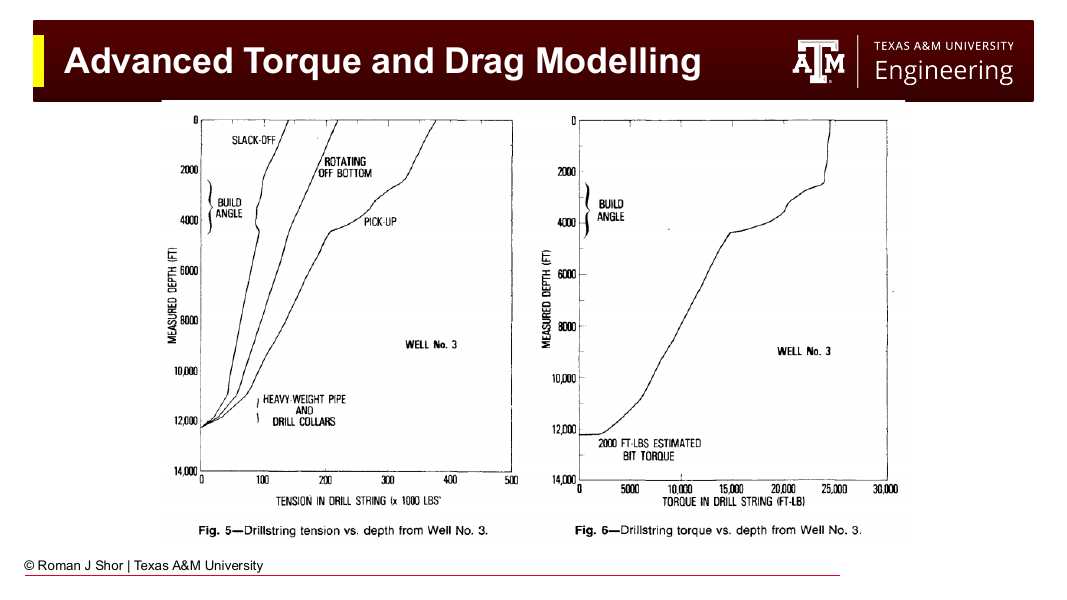
Fig. 179 Model results for a build-and-hold well (Well No. 3 of Johancsik et al., 1984): drillstring tension vs. depth for slack-off, rotating off bottom, and pick-up (left), and torque vs. depth (right). The three hookload curves separate through the build section, where contact forces concentrate; torque accumulates most rapidly there for the same reason.#
13.6 Using Torque and Drag Models in Practice#
13.6.1 Friction Factor Calibration#
The friction factor \(\mu\) is not measured directly — it is calibrated. On each connection or trip, the driller records pick-up weight, slack-off weight, and rotating-off-bottom weight. The engineer runs the model with a range of friction factors and finds the value that reproduces the measured hookloads. Typical calibrated values are roughly 0.15–0.25 in cased hole and 0.25–0.40 in open hole, with water-based muds toward the high end and oil-based muds toward the low end.
The calibrated friction factor is a diagnostic in its own right:
Stable \(\mu\) matching prediction: the well is clean; drilling can proceed.
Rising \(\mu\) trend: deteriorating hole condition — cuttings beds forming, wellbore instability, or developing key seats. The torque and drag model turns routine hookload data into an early-warning system.
Sudden departure: an obstruction, ledge, or pack-off in progress.
13.6.2 Design Applications#
Run in planning mode, the model answers the questions that determine well feasibility:
Can the well be drilled? Slack-off tension must remain positive (no helical buckling lock-up) at every depth to total depth.
Can the casing be run? Casing is heavier and stiffer than drill pipe, with less clearance; slack-off analysis for the casing string frequently governs the maximum reach.
Is the rig adequate? Predicted pick-up hookload sets the hoisting requirement; predicted surface torque sets the top drive requirement (Chapter 3).
Where should tortuosity be spent? Because normal force scales with tension × curvature, doglegs placed deep (where tension is low) are far cheaper than doglegs placed shallow. Trajectory designs that keep the upper hole smooth pay for themselves in reduced torque and drag.
13.7 Beyond the Soft String#
13.7.1 Stiff-String Models#
The soft-string assumption — zero bending stiffness, continuous wall contact — breaks down where the string is stiff relative to the wellbore curvature: BHA components in high-DLS hole, casing in tight doglegs, and any string in hole with significant micro-tortuosity. Stiff-string models (e.g., Tikhonov et al., Dynamic Model for Stiff String Torque and Drag, SPE/IADC Drilling Conference, 2013) add the bending stiffness of the pipe and resolve discrete contact, at the cost of a substantially more complex numerical solution.
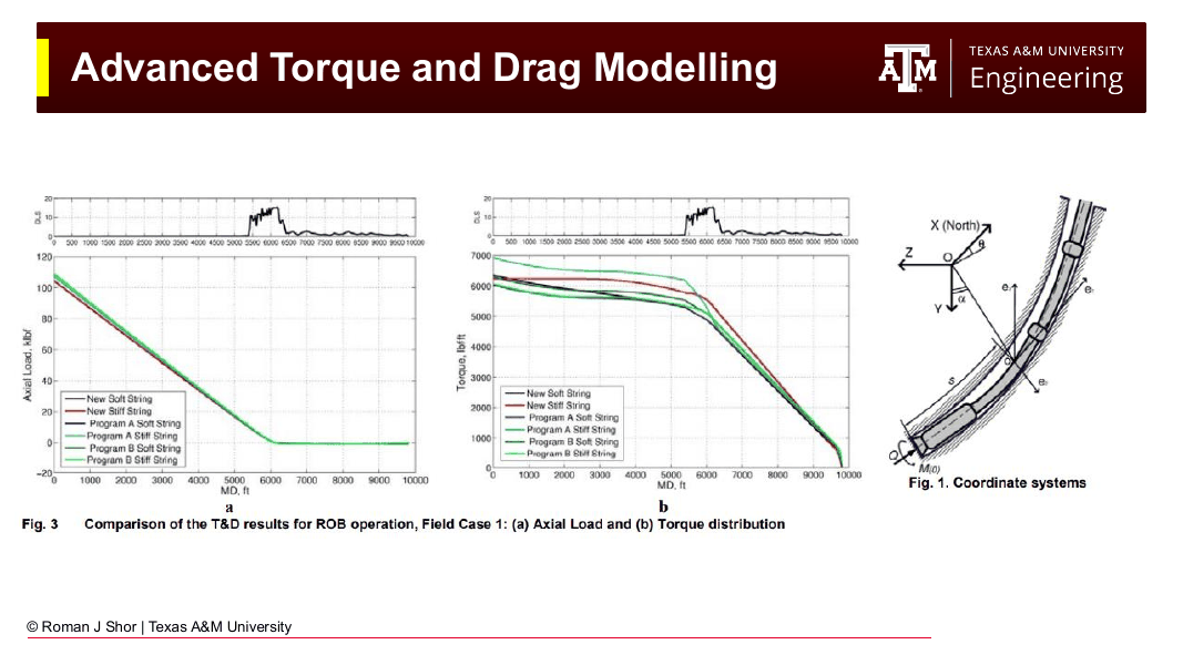
Fig. 180 Soft-string vs. stiff-string model comparison for a field case (after Tikhonov et al., 2013): axial load (left) and torque (right) distributions computed by several commercial soft- and stiff-string implementations. For this well, global tension and torque agree closely across models.#
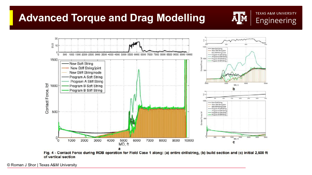
Fig. 181 Where the models differ: local contact force along the string for the same field case. Stiff-string models predict concentrated contact loads through the high-DLS build section (5,500–6,500 ft) that soft-string models smear out — differences that matter for casing wear and fatigue analysis even when hookload predictions agree.#
The practical guidance: soft-string (Johancsik) is adequate — and is the industry default — for hookload and surface torque prediction in most wells. Stiff-string analysis earns its complexity for casing wear studies, high-DLS designs, and buckling-critical extended-reach wells.
13.7.2 Drillstring Vibration#
Torque and drag models are quasi-static: they predict average loads, not dynamics. The rotating drillstring is also an elastic system — recall from Chapter 3 that its aspect ratio makes a violin string look stubby — and it vibrates in three basic modes, all of which reduce drilling performance and damage tools:
Torsional vibration (stick-slip): a cyclic buildup and release of torque driven by the nonlinear friction at the bit. Surface RPM remains nearly constant while downhole RPM oscillates between zero and two to three times the surface value; at surface it appears as an oscillating torque signal.
Lateral vibration (whirl): the string or bit orbits the borehole rather than rotating on center, generating high-frequency impact loads.
Axial vibration (bit bounce): driven by bit-rock interaction, capable of exciting natural frequencies of the string.
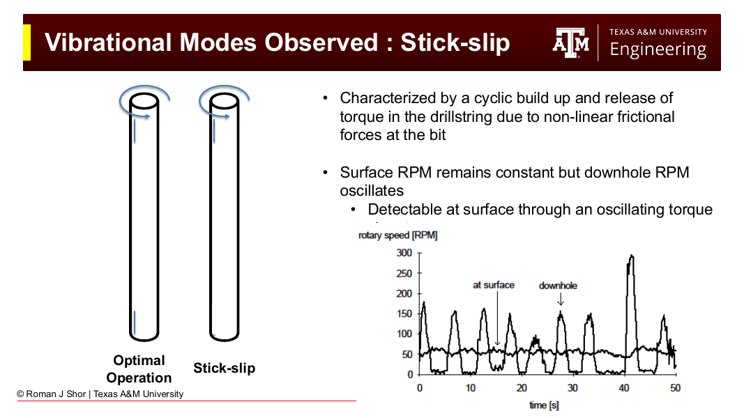
Fig. 182 Stick-slip: surface rotary speed is nearly constant while downhole RPM oscillates between zero and roughly three times the surface speed — the signature of torsional vibration, detectable at surface as oscillating torque.#
Mitigation combines operating practice (the parameter management discussed with drilling performance later in this text) with control engineering: modern top drives use tuned speed controllers that absorb torsional oscillations rather than stiffly regulating RPM, substantially reducing stick-slip severity. The interaction of friction, trajectory, and dynamics remains an active research area — and a reason the torque and drag model of this chapter is a foundation rather than the final word.
Chapter Summary#
The minimum curvature method computes 3D wellbore position from survey data by assuming a circular arc between stations in the plane of the two survey vectors. The dogleg angle \(\beta\) captures the total angular change (inclination and azimuth together), the ratio factor \(RF = (2/\beta)\tan(\beta/2)\) corrects the chord average for curvature, and the position increments follow directly. It is the industry standard for both planning and survey evaluation.
Torque and drag arise from Coulomb friction at drillstring-wellbore contact. The Johancsik soft-string model treats the string as a flexible cable and marches from the bit to surface: for each element, the normal force \(F_n = \sqrt{(F_t \Delta\alpha \sin\bar{\theta})^2 + (F_t \Delta\theta + W\sin\bar{\theta})^2}\) combines curvature and gravity contributions; tension changes by \(\Delta F_t = W\cos\bar{\theta} \pm \mu F_n\) (sign set by pick-up vs. slack-off, zero axial friction while rotating); and torque accumulates as \(\Delta M = \mu F_n r\). Friction factors are calibrated against measured pick-up, slack-off, and rotating hookloads, and the calibrated trend is itself a hole-condition diagnostic.
Soft-string analysis is the industry default; stiff-string models add bending stiffness where local contact forces matter (casing wear, high DLS, buckling-critical designs). Beyond the quasi-static picture, the drillstring vibrates torsionally (stick-slip), laterally (whirl), and axially — dynamics that set the ultimate limits on drilling performance in deviated wells.
Key Equations#
Quantity |
Formula |
|---|---|
Dogleg angle |
\(\beta = \cos^{-1}[\cos(I_2 - I_1) - \sin I_1 \sin I_2 (1 - \cos(Az_2 - Az_1))]\) |
Dogleg severity |
\(\text{DLS} = \beta_\text{deg} \times 100 / \Delta MD\) |
Ratio factor |
\(RF = (2/\beta)\tan(\beta/2)\) |
ΔTVD (MCM) |
\((\Delta MD/2)(\cos I_1 + \cos I_2) \times RF\) |
ΔNorth (MCM) |
\((\Delta MD/2)(\sin I_1 \cos Az_1 + \sin I_2 \cos Az_2) \times RF\) |
ΔEast (MCM) |
\((\Delta MD/2)(\sin I_1 \sin Az_1 + \sin I_2 \sin Az_2) \times RF\) |
Normal force (Johancsik) |
\(F_n = \sqrt{(F_t \Delta\alpha \sin\bar{\theta})^2 + (F_t \Delta\theta + W\sin\bar{\theta})^2}\) |
Tension increment |
\(\Delta F_t = W\cos\bar{\theta} \pm \mu F_n\) |
Torque increment |
\(\Delta M = \mu F_n r\) |
Practice Problems#
13.1 Two survey stations read: Station 1 — MD 8,200 ft, inclination 62°, azimuth 155°; Station 2 — MD 8,295 ft, inclination 65°, azimuth 149°.
(a) Compute the dogleg angle \(\beta\) and the dogleg severity. (b) Compute the ratio factor. (c) Compute ΔTVD, ΔNorth, and ΔEast for the interval. (d) Recompute the dogleg severity ignoring the azimuth change. What fraction of the true curvature would be missed?
13.2 A well plan calls for a maximum DLS of 3°/100 ft. Surveys come in at MD 6,000 ft (I = 20°, Az = 75°) and MD 6,100 ft (I = 22°, Az = 82°). Is the well within specification? Show your calculation.
13.3 A drillstring element in a build section has: buoyed weight \(W = 2{,}000\) lb, average inclination 45°, \(\Delta\theta = 5°\) (no azimuth change), tension at the lower end \(F_t = 120{,}000\) lb, \(\mu = 0.30\), contact radius \(r = 0.19\) ft.
(a) Compute the normal force \(F_n\) and identify the fraction contributed by tension-through-curvature vs. gravity. (b) Compute the tension at the top of the element for pick-up and for slack-off. (c) Compute the torque increment while rotating. (d) The same element is moved to a depth where the tension below it is only 20,000 lb. Recompute (a)–(c) and comment on why dogleg placement in a well design matters.
13.4 During a trip at 12,000 ft MD, the driller records: pick-up weight 385,000 lb, slack-off weight 265,000 lb, rotating-off-bottom weight 325,000 lb.
(a) Which measurement best approximates the true buoyed string weight, and why? (b) Estimate the total axial drag during pick-up and during slack-off. (c) On the next trip a week later, pick-up weight has risen to 410,000 lb with the same string and mud. List three possible causes and one diagnostic step for each.
13.5 Explain in your own words:
(a) Why the soft-string model requires the wellpath from the minimum curvature method as its geometric input. (b) Why the axial friction term vanishes while rotating, and how drillers exploit this when tripping through a high-drag well. (c) Why a stiff-string model may predict nearly the same hookload as a soft-string model yet very different casing wear. (d) Why slack-off tension going negative in the model flags a well that may not reach its planned total depth.
References#
Johancsik, C.A., Friesen, D.B., and Dawson, R., “Torque and Drag in Directional Wells — Prediction and Measurement,” Journal of Petroleum Technology, June 1984.
Tikhonov, V., Valiullin, K., Nurgaliev, A., et al., “Dynamic Model for Stiff String Torque and Drag,” SPE/IADC Drilling Conference, 2013.
Mitchell, R.F. and Miska, S.Z. (eds.), Fundamentals of Drilling Engineering, Society of Petroleum Engineers, 2011.