Chapter 6: Drilling Fluid Calculations

Learning Objectives

By the end of this chapter, you will be able to:

• Convert between common oilfield units for density, pressure, and volume

• Apply the ideal mixing model to calculate the density of a multi-component mud system

• Explain why the ideal mixing model does not apply to dissolved salts

• Calculate the quantity of barite required to increase mud weight to a target value

• Calculate the volumes of water (or base fluid) required to dilute a mud to a target density

• Calculate hydrostatic and flowing bottomhole pressures, including equivalent circulating density (ECD)

• Interpret the physical meaning of calculated rheological parameters

---

6.1 Introduction

Chapters 4 and 5 built the conceptual foundation for understanding drilling fluids: what they do, how they are classified, and how their properties are measured. This chapter bridges that foundation to engineering practice: the calculations that a drilling engineer and mud engineer perform routinely to design, maintain, and adjust a mud system.

The calculations in this chapter fall into two categories:

1. Density calculations — How do we design a mud to a target density? How much barite do we add to weight up? How much water to dilute? What pressure does the mud column exert at depth?

2. Rheology calculations — Given a set of Fann viscometer readings, how do we calculate the parameters of each rheological model, and what do those parameters tell us about the fluid?

Getting these calculations right matters. A mud that is too light risks a kick; a mud that is too heavy risks fracturing the formation. These are not hypothetical concerns — they are the daily operational reality of drilling engineering.

---

6.2 Oilfield Units

Drilling calculations use a mixture of SI and US customary units. The oilfield has its own unit conventions that are deeply embedded in practice, even as the global industry has partially moved toward SI. A drilling engineer must be fluent in both systems and, critically, must never confuse them.

6.2.1 Key Unit Conversions

Table 1 Common oilfield unit conversions for drilling fluid calculations

Quantity	Oilfield Unit	SI Unit	Conversion
Density	ppg (lb/gal)	kg/m³	1 ppg = 119.8 kg/m³
Density	ppg (lb/gal)	g/cm³ (SG)	1 ppg = 0.1198 SG
Pressure	psi	kPa	1 psi = 6.895 kPa
Pressure gradient	psi/ft	kPa/m	1 psi/ft = 22.62 kPa/m
Volume	barrel (bbl)	m³	1 bbl = 0.1590 m³
Volume	barrel (bbl)	US gallons	1 bbl = 42 US gal
Mass (solids)	sack (sk)	kg	1 sack barite = 100 lb = 45.4 kg
Viscosity	centipoise (cP)	mPa·s	1 cP = 1 mPa·s (exact)
Shear stress	lb/100 ft²	Pa	1 lb/100 ft² = 0.4788 Pa

6.2.2 The Hydrostatic Pressure Equation in Oilfield Units

The fundamental pressure equation in oilfield units is:

\[\boxed{P_h \text{ (psi)} = 0.052 \times \rho \text{ (ppg)} \times D \text{ (ft)}}\]

The factor 0.052 consolidates the unit conversions: 1 ppg = 0.052 psi/ft. This coversion is used constantly: many pressure calculations in drilling start here.

Key Term: Equivalent Mud Weight (EMW)

Equivalent mud weight (EMW), also called equivalent density, expresses a pressure as the density of a fluid column that would produce that pressure at a given depth. It allows pressures (pore pressure, fracture pressure, annular friction pressure) to be compared on the same scale as mud weight:

\[\text{EMW (ppg)} = \frac{P \text{ (psi)}}{0.052 \times D \text{ (ft)}}\]

---

6.3 The Ideal Mixing Model for Mud Density

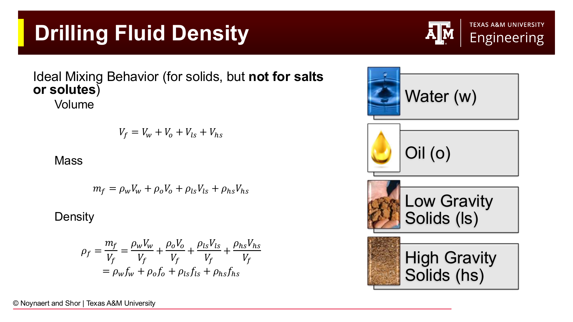
Fig. 69 The ideal mixing model for drilling fluid density. Volumes of each component add directly (volume additivity); masses add directly (mass additivity); density is the ratio of total mass to total volume.

6.3.1 Derivation

The ideal mixing model assumes that when solid particles are added to a liquid, the total volume of the mixture equals the sum of the individual component volumes, and similarly for mass. This is a good approximation for suspensions of solids in liquids, where the solid particles occupy distinct physical space.

For a mud containing water (\(w\)), oil (\(o\)), low-gravity solids (\(ls\)), and high-gravity solids (\(hs\)):

Volume additivity: $\(V_f = V_w + V_o + V_{ls} + V_{hs}\)$

Mass balance: $\(m_f = \rho_w V_w + \rho_o V_o + \rho_{ls} V_{ls} + \rho_{hs} V_{hs}\)$

Fluid density (mass divided by volume): $\(\rho_f = \frac{m_f}{V_f} = \rho_w f_w + \rho_o f_o + \rho_{ls} f_{ls} + \rho_{hs} f_{hs}\)$

where \(f_i = V_i / V_f\) is the volume fraction of component \(i\), and \(\sum f_i = 1\).

This can also be written as:

\[\rho_f = \sum_i \rho_i f_i\]

In other words: the density of the mixture is the volume-weighted average of the component densities. This is the central equation for all mud density design calculations.

6.3.2 ⚠️ Important Limitation: Ideal Mixing Does NOT Apply to Dissolved Salts

Warning: Salts dissolve and do not follow ideal mixing behavior

The ideal mixing model assumes volume additivity — that adding a component increases the total volume. This is true for solid particles (barite, drill cuttings, bentonite) which physically occupy space.

It is NOT true for dissolved salts. When salt dissolves in water, the ions insert themselves into the existing molecular structure of the water, causing only a small increase in volume that is much less than the volume of the dry salt crystals. Adding 1 kg of NaCl to 1 liter of water does NOT produce 1 liter + volume of NaCl. The volume increases by much less than expected.

For dissolved salt systems (brines), density is determined from brine density tables or correlations (see Section 6.4), not from the ideal mixing model.

6.3.3 Standard Component Densities

For ideal mixing calculations, the following standard densities apply:

Component	Typical Density (SG)	Density (ppg)
Fresh water	1.00	8.34
Seawater	1.03–1.05	8.59–8.76
Diesel oil	0.84	7.0
Mineral oil	0.80–0.85	6.67–7.09
Synthetic base oil (paraffin)	0.79–0.81	6.59–6.76
Bentonite	2.60	21.7
Drill solids (average)	2.60	21.7
Barite (BaSO₄)	4.20	35.0
Hematite (Fe₂O₃)	5.10	42.5

---

6.4 Density from Dissolved Salts

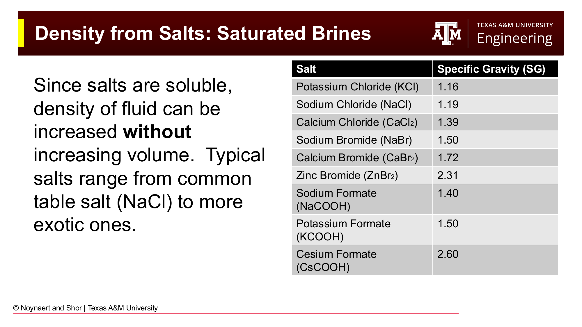
Fig. 70 Maximum achievable specific gravity of saturated brines from common oilfield salts. Because dissolved salts do not add proportional volume, densities significantly higher than fresh water can be achieved without any solid particles.

Dissolved salts increase brine density beyond that of fresh water. Because the ions occupy interstitial space in the water structure, the increase in density is greater per unit mass than the ideal mixing model would predict. The density of a brine is typically read from tabulated data or calculated using empirical correlations specific to each salt/concentration combination.

Common oilfield brines and their maximum saturated densities:

Salt	Maximum SG (saturated)	Maximum (ppg)
Potassium Chloride (KCl)	1.16	9.67
Sodium Chloride (NaCl)	1.19	9.92
Calcium Chloride (CaCl₂)	1.39	11.60
Sodium Bromide (NaBr)	1.50	12.52
Calcium Bromide (CaBr₂)	1.72	14.35
Zinc Bromide (ZnBr₂)	2.31	19.27
Sodium Formate (NaCOOH)	1.40	11.68
Potassium Formate (KCOOH)	1.50	12.52
Cesium Formate (CsCOOH)	2.60	21.70

Brines are particularly important for:

• Completion and workover fluids — where no solids can be present to damage the reservoir. A CaCl₂ or CaBr₂ brine can provide up to 11.6–14.4 ppg density without any solids.

• Deepwater riser-less drilling of the top-hole section, where lightweight brine is used instead of conventional mud to reduce fracture risk in shallow, low-fracture-gradient formations. In riser-less drilling, drilling fluids are discharged directly into the ocean at the sea floor.

• Formate brines (sodium, potassium, and cesium formate) — premium brines used in HPHT applications. Cesium formate can reach 21.7 ppg — the highest achievable density for a clear brine — and is also environmentally benign.

---

6.5 Density from Solid Weighting Agents

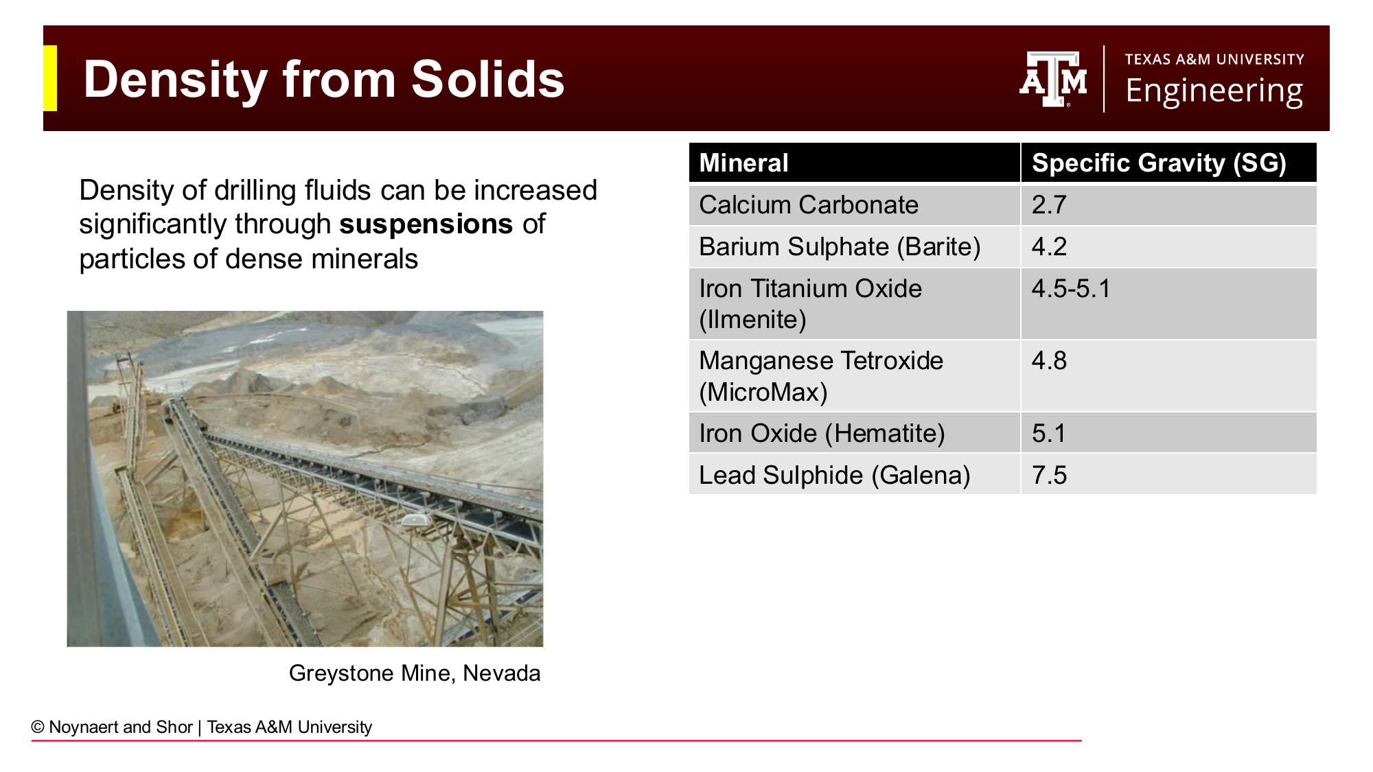
Fig. 71 Solid weighting agents used in drilling fluids, ranked by specific gravity. Barite is the industry standard; higher-density agents are used when minimum solids volume is required (e.g., to maintain low viscosity at very high mud weights).

Weighting Agent	Chemical Formula	SG	Max achievable MW (ppg))	Notes
Calcium Carbonate	CaCO₃	2.7	~11.5	Acid-soluble; used in reservoir sections
Barite	BaSO₄	4.2	~22	Industry standard; chemically inert
Ilmenite	FeTiO₃	4.5–5.1	~22+	Alternative to barite; lower fine-particle content
Manganese Tetroxide (MicroMax)	Mn₃O₄	4.8	~22+	Fine particle; low viscosity at high MW
Hematite	Fe₂O₃	5.1	~23	Higher density than barite; harder particles
Galena	PbS	7.5	~26	Very high density; rarely used; toxicity concerns

Barite dominates the industry because it is inert (does not react with formation fluids or mud additives), relatively inexpensive, globally available, and provides adequate maximum density for the majority of wells. Its low hardness (3 on the Mohs scale) reduces abrasive wear on pump components and drill bits compared to harder minerals.

The maximum practically achievable mud weight with barite-weighted WBM is approximately 22 ppg. At this density, the solids volume fraction is so high that the mud becomes difficult to pump and filter cakes become extremely thick. Hematite is sometimes used above 19–20 ppg to achieve slightly lower solids volumes at the same density.

---

6.6 Mud Density Design Calculations

6.6.1 The General Mixing Equation

For a two-component system (i.e., an existing mud being adjusted by adding a weighting agent or diluent), the ideal mixing model gives:

\[\rho_2 = \frac{m_1 + m_{add}}{V_1 + V_{add}} = \frac{\rho_1 V_1 + \rho_{add} V_{add}}{V_1 + V_{add}}\]

where subscript 1 denotes the original mud, subscript 2 denotes the final mud, and subscript \(add\) denotes the material being added.

For the common case of adding barite (or any solid weighting agent) to an existing mud:

\[\rho_2 (V_1 + V_{bar}) = \rho_1 V_1 + \rho_{bar} V_{bar}\]

Solving for the volume of barite to add per unit volume of original mud:

\[\frac{V_{bar}}{V_1} = \frac{\rho_2 - \rho_1}{\rho_{bar} - \rho_2}\]

Or, solving for the volume of barite to add to achieve density \(\rho_2\) in a final volume \(V_2\):

\[V_{bar} = \frac{V_2 (\rho_2 - \rho_1)}{\rho_{bar} - \rho_1}\]

6.6.2 Converting Between Volume and Mass of Barite

In the field, barite is supplied in sacks (100 lb each). The volume of one sack of barite:

\[V_{1\,\text{sack}} = \frac{100 \text{ lb}}{35.0 \text{ ppg}} = 2.857 \text{ gal} = 0.0680 \text{ bbl}\]

So, the number of sacks of barite per barrel of mud added is:

\[\text{Sacks/bbl} = \frac{V_{bar}/V_1 \text{ (gal/gal)}}{0.0680 \text{ bbl/sack}} \times \frac{1 \text{ bbl}}{42 \text{ gal}}\]

This is simplified in most oilfield references to the formula:

\[\text{Sacks barite per barrel of new mud} = \frac{1{,}470(\rho_2 - \rho_1)}{35 - \rho_2}\]

where densities are in ppg.

6.6.3 Diluting with Water (or Base Oil)

To reduce mud density by adding water (density \(\rho_w = 8.34\) ppg):

\[\frac{V_w}{V_1} = \frac{\rho_1 - \rho_2}{\rho_2 - \rho_w}\]

6.6.4 Simultaneous Dilution and Weighting

Sometimes the mud density needs to be maintained while increasing total volume (to fill a larger hole after running casing). Or, the mud needs to be thinned by dilution but must then be re-weighted back up. These simultaneous problems require solving two equations:

• Volume balance: \(V_1 + V_w + V_{bar} = V_2\)

• Mass balance: \(\rho_1 V_1 + \rho_w V_w + \rho_{bar} V_{bar} = \rho_2 V_2\)

Two equations, two unknowns (\(V_w\) and \(V_{bar}\)), given \(V_1\), \(V_2\), and all three densities.

---

6.7 Effects of Temperature and Pressure on Mud Density

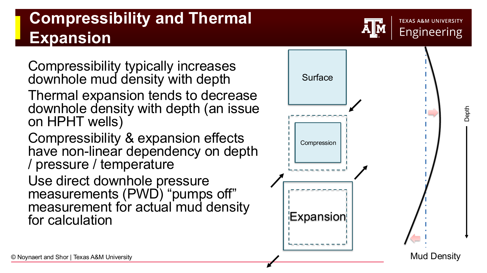
Fig. 72 Competing effects of compressibility and thermal expansion on mud density with depth. Compressibility increases density; thermal expansion decreases it. On most wells these effects roughly offset each other, but on HPHT wells the thermal expansion of oil can significantly reduce downhole density below its surface-measured value.

The mud weight measured at surface using a mud balance is not necessarily the density of the mud at depth. Two effects cause the downhole density to differ from the surface measurement:

Compressibility — As mud is pressurized with increasing depth, the liquid phase compresses slightly, increasing its density. For the water phase, this effect is small (water is nearly incompressible). For oil and synthetic base fluids, compressibility is more significant.

Thermal expansion — As mud temperature increases with depth (following the geothermal gradient), the liquid phase expands, decreasing its density. For oil and synthetic base fluids, thermal expansion is substantial — a typical synthetic base fluid expands 5–8% between surface conditions and HPHT downhole conditions. This can reduce the effective downhole density of an OBM/SBM by 0.3–0.8 ppg below the surface mud weight measurement.

On most standard wells, compressibility and thermal expansion partially offset each other and the surface-measured mud weight is a reasonable approximation of downhole density. On HPHT wells (high pressure, high temperature — typically defined as > 10,000 psi and > 300°F at bottomhole), these effects can be large enough to cause well control problems if not explicitly accounted for in the mud weight design.

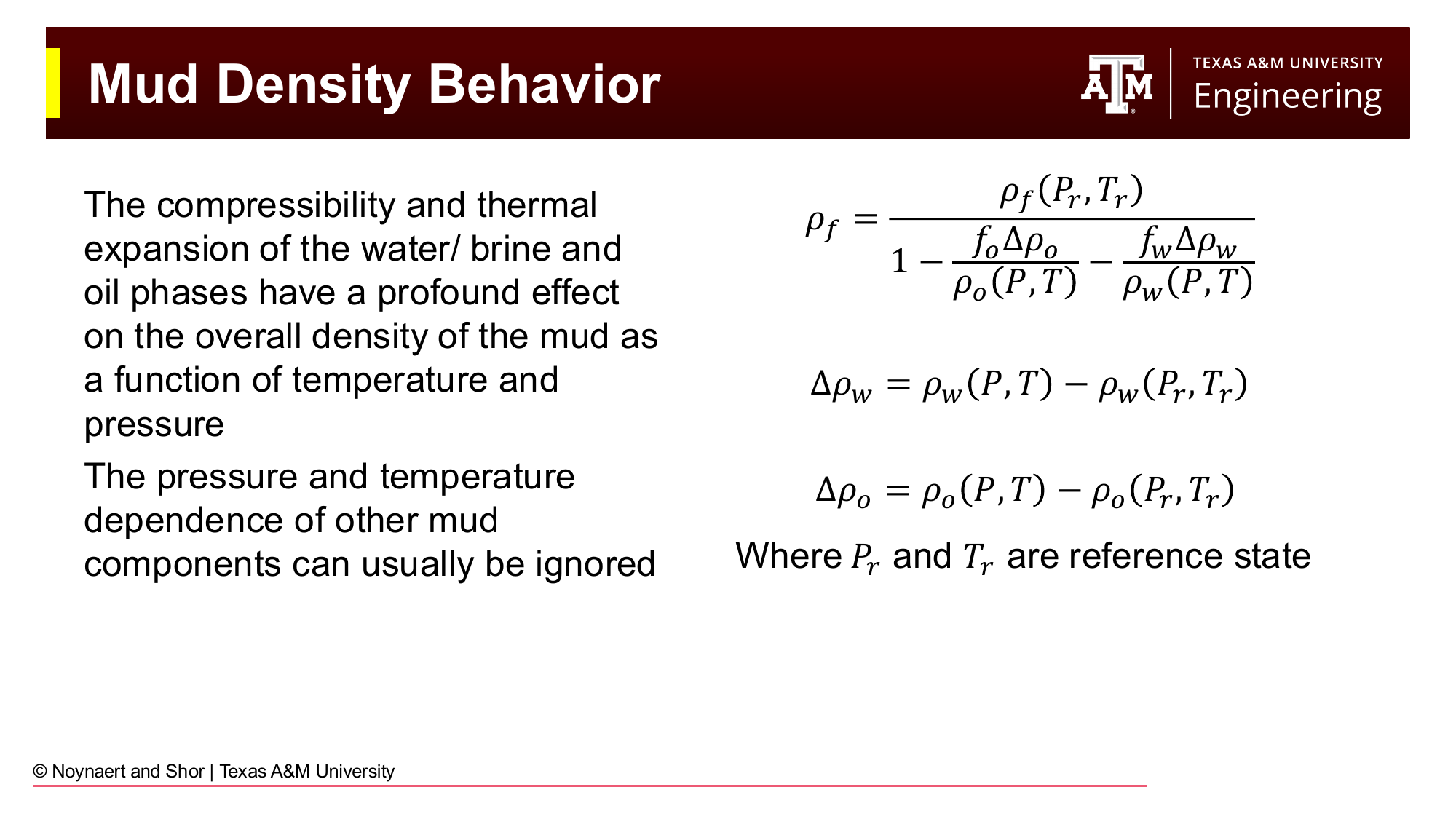
Fig. 73 The general equation for mud density as a function of temperature and pressure, accounting for the compressibility and thermal expansion of the water and oil phases. For most wells, the simpler hydrostatic equation using surface mud weight gives an adequate approximation.

For most routine well planning, the surface mud weight is used directly in the hydrostatic pressure equation. For HPHT applications, density should be corrected using the PVT (pressure-volume-temperature) behavior of the base fluid components. Alternatively, pressure-while-drilling (PWD) tools provide direct downhole pressure measurements, eliminating the need for modeled density corrections.

---

6.8 Hydrostatic Pressure

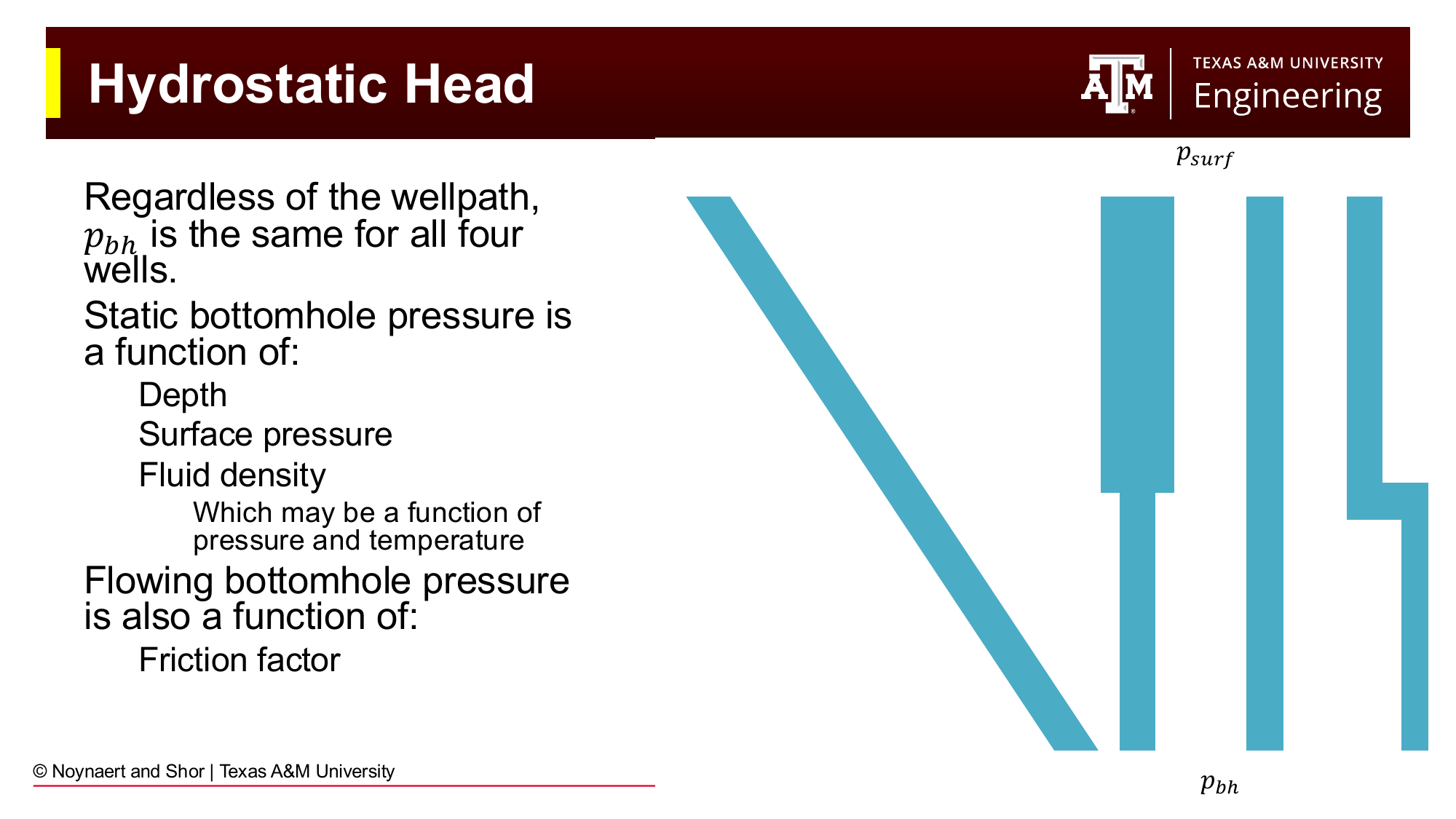
Fig. 74 Hydrostatic pressure depends only on the true vertical depth (TVD) of the fluid column, not on the wellpath. All four wells shown have the same bottomhole pressure because the TVD and fluid density are the same.

The hydrostatic (static) pressure at any point in the wellbore is determined solely by the true vertical depth (TVD) of the fluid column above that point and the density of the fluid. The path of the wellbore — whether vertical, deviated, or horizontal — does not affect the hydrostatic pressure calculation, because pressure is determined by the vertical height of the fluid column, not its length along the wellbore.

Static bottomhole pressure:

\[P_{bh} = P_{surf} + \int_0^{TVD} \rho_f(x, P(x), T(x))\, dx\]

For a uniform mud density with negligible surface pressure (which is the usual assumption):

\[\boxed{P_{bh} \text{ (psi)} = 0.052 \times \rho_f \text{ (ppg)} \times TVD \text{ (ft)}}\]

6.8.1 The U-Tube Model

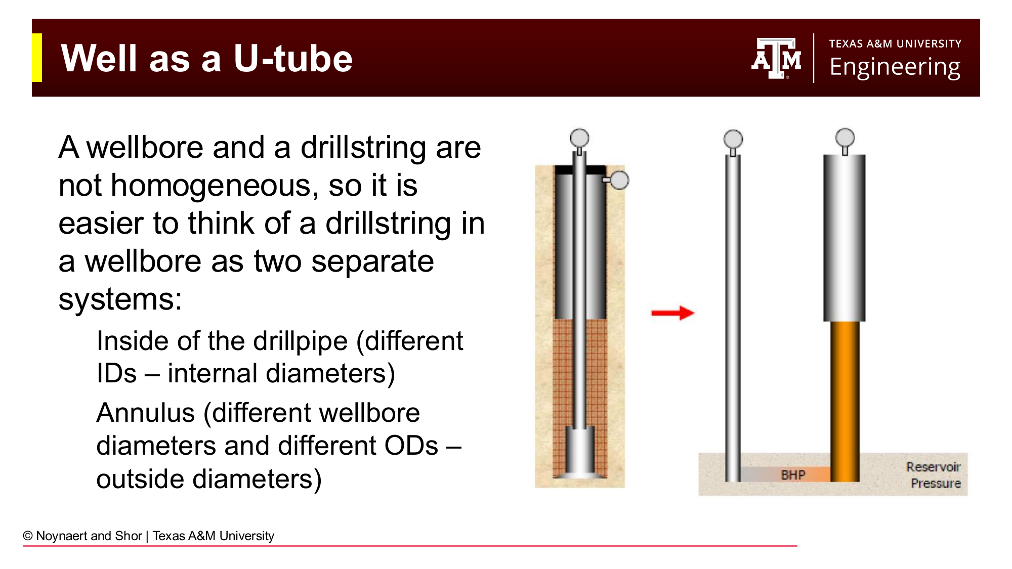
Fig. 75 The wellbore-drillstring system viewed as a U-tube. The drill string interior (left leg) and the annulus (right leg) may contain fluids of different densities and are connected at the bit. The pressure at the bit must balance from both sides.

It is useful to model a wellbore and drill string as a U-tube: two connected columns of fluid. The drill string interior and the annulus are the two legs, connected at the bit. At any connected point, the pressure from both sides must be equal.

This model is essential for:

• Kick detection — if formation fluid enters the annulus (lower density than mud), the pressure balance shifts

• Tripping calculations — the pressure at the bottom of the hole changes as pipe is added or removed

• Cement displacement — designing the pump rates to maintain balanced pressure during cementing operations

In the U-tube, the pressure at the bit (\(P_{bit}\)) must equal the hydrostatic pressure in the drillstring minus any surface pump pressure, and must also equal the pressure from the annular side:

\[P_{surf,pump} + \rho_{dp} \times 0.052 \times TVD = \rho_{ann} \times 0.052 \times TVD + P_{formation}\]

---

6.9 Flowing Bottomhole Pressure and ECD

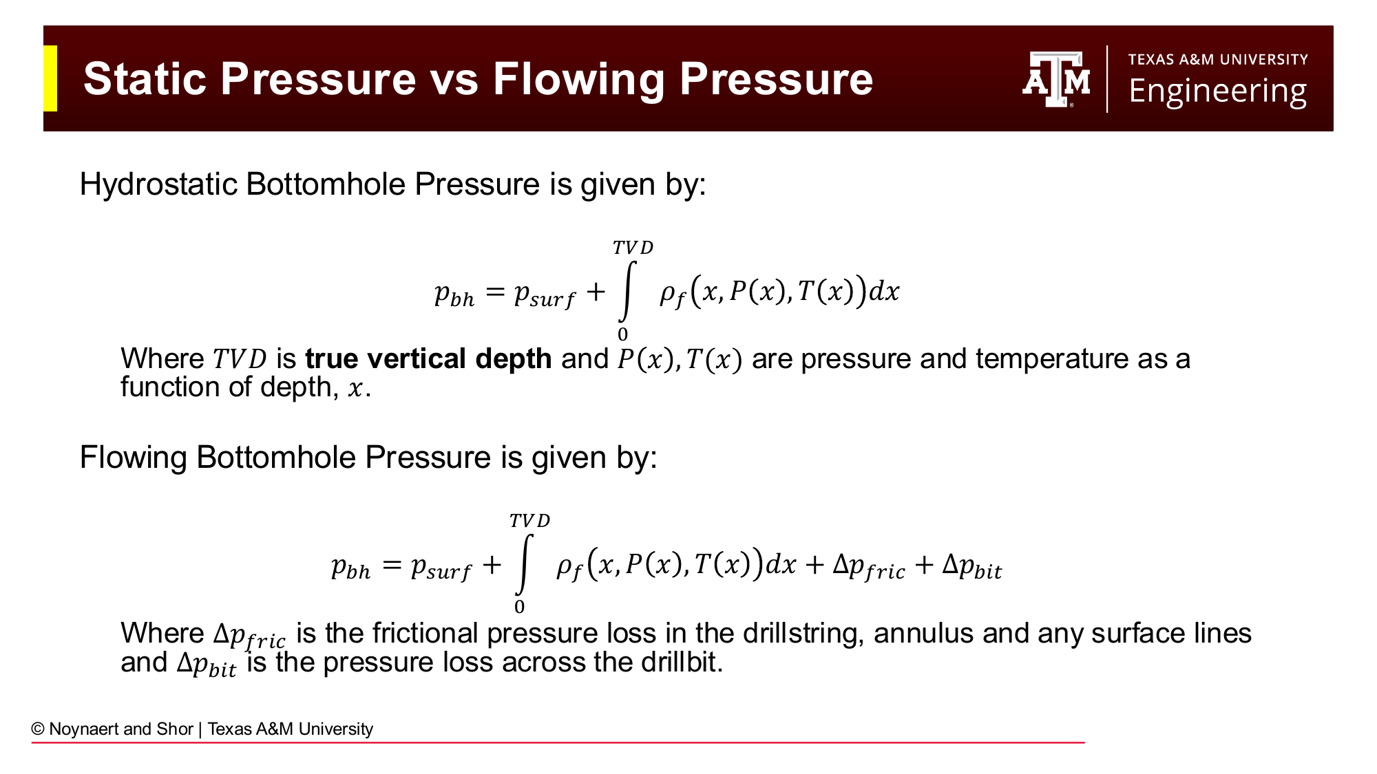
Fig. 76 Static vs. flowing bottomhole pressure. When the mud pumps are running, friction pressure losses in the annulus add to the hydrostatic pressure, increasing the effective pressure on the formation. This additional pressure is the basis for the equivalent circulating density (ECD).

When the mud pumps are running and the mud is circulating, additional pressure is generated by friction as the fluid flows through the drill string and annulus. The flowing bottomhole pressure exceeds the static (hydrostatic) bottomhole pressure:

\[P_{bh,flowing} = P_{surf} + P_{hydrostatic} + \Delta P_{friction} + \Delta P_{bit}\]

where:

• \(\Delta P_{friction}\) = frictional pressure loss in the drill string, annulus, and surface lines

• \(\Delta P_{bit}\) = pressure drop across the drill bit nozzles

The increased bottomhole pressure while circulating is expressed as the equivalent circulating density (ECD):

\[\boxed{\text{ECD (ppg)} = \rho_{mud} + \frac{\Delta P_{ann} \text{ (psi)}}{0.052 \times TVD \text{ (ft)}}}\]

where \(\Delta P_{ann}\) is the frictional pressure loss in the annulus (not including the bit or drillstring interior).

Key Term: Equivalent Circulating Density (ECD)

ECD is the effective density that, at the given TVD, would produce the same bottomhole pressure as the actual mud weight plus all annular friction pressure losses. It represents the total pressure exerted on the formation while circulating. The ECD must remain below the fracture gradient throughout the open hole to avoid lost circulation. In wells with narrow drilling windows, ECD management is a critical operational challenge.

Swab and surge pressures are transient equivalents:

• Surge (tripping in): running the drill string into the hole creates a positive pressure pulse at the bit, temporarily increasing bottomhole pressure above hydrostatic. Too fast tripping-in can fracture a weak formation.

• Swab (tripping out): pulling the drill string creates a negative pressure pulse, temporarily reducing bottomhole pressure below hydrostatic. Too fast tripping-out can induce a kick.

Both surge and swab pressures increase with pipe speed and mud viscosity, and decrease with larger annular clearances.

---

6.10 Rheology Calculations: Complete Formulas

This section collects all four rheological model calculations in one place for reference. Each model is calculated from readings of the Fann VG/35 viscometer, which measures dial deflection (\(\theta_N\)) at rotor speeds of 600, 300, 200, 100, 6, and 3 rpm.

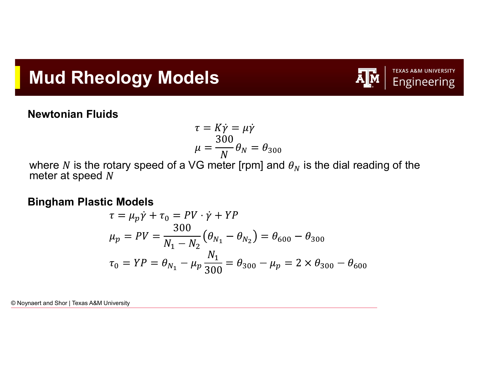
Fig. 77 Fann viscometer conversion factors and Bingham Plastic model formulas. PV and YP are the two most commonly reported mud rheology parameters.

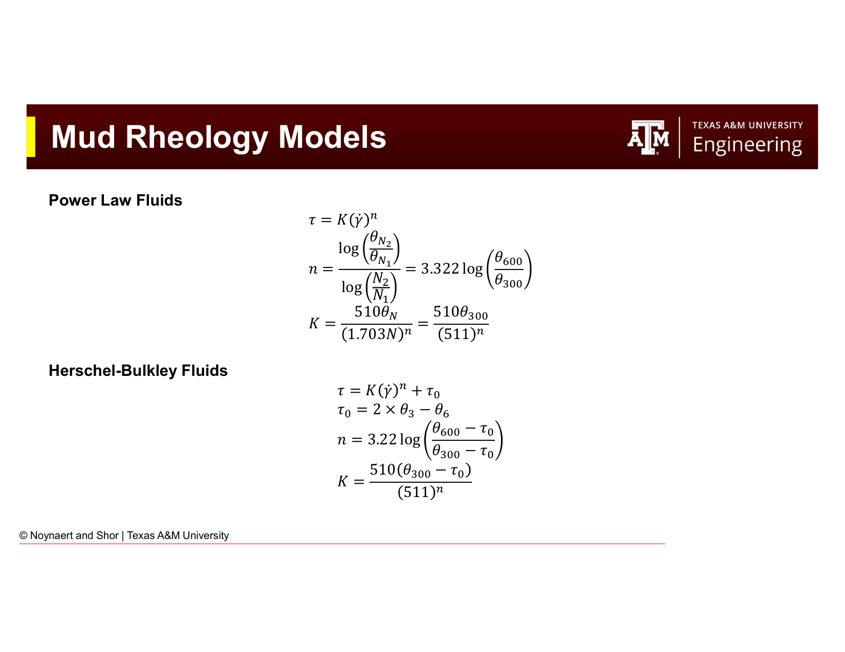
Fig. 78 Power Law and Herschel-Bulkley model formulas from Fann readings. The HB model requires the 3 and 6 rpm readings (low-shear-rate readings) to establish the yield stress.

6.10.1 Fann Viscometer Conversion Factors

The Fann meter geometry converts instrument readings to physical units:

\[\dot{\gamma} \text{ (s}^{-1}\text{)} = 1.703 \times N \text{ (rpm)}\]

\[\tau \text{ (lb/100 ft}^2\text{)} \approx \theta_N \quad \text{(1 dial unit ≈ 1.067 lb/100 ft}^2\text{)}\]

6.10.2 Newtonian Model

\[\tau = \mu \dot{\gamma}\]

\[\mu \text{ (cP)} = \frac{300 \cdot \theta_N}{N}\]

Use any single speed (typically 600 rpm). If the fluid is truly Newtonian, all speeds should give the same \(\mu\).

6.10.3 Bingham Plastic Model

\[\tau = PV \cdot \dot{\gamma} + YP\]

\[PV \text{ (cP)} = \theta_{600} - \theta_{300}\]

\[YP \text{ (lb/100 ft}^2\text{)} = \theta_{300} - PV = 2\theta_{300} - \theta_{600}\]

Apparent viscosity at 600 rpm (cP):

\[AV = \frac{\theta_{600}}{2}\]

6.10.4 Power Law Model

\[\tau = K \dot{\gamma}^n\]

\[n = 3.322 \log\left(\frac{\theta_{600}}{\theta_{300}}\right)\]

\[K \text{ (mPa·s}^n\text{)} = \frac{510 \cdot \theta_{300}}{511^n}\]

\(n = 1\) for a Newtonian fluid; \(n < 1\) for shear-thinning (typical for drilling muds).

6.10.5 Herschel-Bulkley Model

\[\tau = K \dot{\gamma}^n + \tau_0\]

\[\tau_0 \text{ (lb/100 ft}^2\text{)} = 2\theta_3 - \theta_6\]

\[n = 3.322 \log\left(\frac{\theta_{600} - \tau_0}{\theta_{300} - \tau_0}\right)\]

\[K = \frac{510(\theta_{300} - \tau_0)}{511^n}\]

Requires 3 and 6 rpm readings in addition to 600 and 300 rpm.

6.10.6 Gel Strengths

Parameter	Symbol	Reading
10-second gel strength	\(G_{10s}\)	Max dial reading at 3 rpm after 10 s rest
10-minute gel strength	\(G_{10m}\)	Max dial reading at 3 rpm after 10 min rest
30-minute gel strength	\(G_{30m}\)	Max dial reading at 3 rpm after 30 min rest

Units: lb/100 ft². Flat gels: \(G_{10m} \approx G_{10s}\). Progressive gels: \(G_{30m} \gg G_{10s}\).

---

Worked Examples

Example 6.1 — Mud Density from Components (Ideal Mixing)

Problem: A mud engineer is preparing a fresh WBM from the following components. Calculate the density of the resulting mud.

Component	Volume added
Fresh water	0.800 bbl
Bentonite	0.030 bbl
Barite	0.050 bbl

Solution:

Step 1: Find component densities (from standard table)

Component	Volume (bbl)	Density (ppg)	Density (lb/bbl)
Fresh water	0.800	8.34	350.3
Bentonite	0.030	21.7	911.4
Barite	0.050	35.0	1,470

Note: 1 bbl = 42 gal, so density in lb/bbl = density in ppg × 42

Step 2: Total volume and total mass

\[V_f = 0.800 + 0.030 + 0.050 = 0.880 \text{ bbl}\]

\[m_f = (0.800)(350.3) + (0.030)(911.4) + (0.050)(1{,}470)\]

\[= 280.2 + 27.3 + 73.5 = 381.0 \text{ lb}\]

Step 3: Fluid density

\[\rho_f = \frac{381.0 \text{ lb}}{0.880 \text{ bbl} \times 42 \text{ gal/bbl}} = \frac{381.0}{36.96} = \boxed{10.3 \text{ ppg}}\]

---

Example 6.2 — Weighting Up with Barite

Problem: A drilling crew has 500 bbl of 10.0 ppg WBM in their active pit. They need to increase the mud weight to 12.5 ppg before drilling into a high-pressure zone.

(a) How many barrels of barite must be added?
(b) How many 100-lb sacks of barite does this represent?
(c) What will the final mud volume be?

Solution:

(a) Volume of barite to add:

Using the weighting formula:

\[V_{bar} = \frac{V_1 (\rho_2 - \rho_1)}{\rho_{bar} - \rho_2} \times \frac{1}{\text{(implicit in the derivation — actually:)}}\]

From the mixing equation (solving for \(V_{bar}\) given \(V_1 = 500\) bbl, \(\rho_1 = 10.0\), \(\rho_2 = 12.5\), \(\rho_{bar} = 35.0\) ppg):

\[V_{bar} = \frac{V_1 (\rho_2 - \rho_1)}{\rho_{bar} - \rho_2} = \frac{500 \times (12.5 - 10.0)}{35.0 - 12.5} = \frac{500 \times 2.5}{22.5} = \boxed{55.6 \text{ bbl of barite}}\]

(b) Number of sacks:

Mass of barite: \(55.6 \text{ bbl} \times 42 \text{ gal/bbl} \times 35.0 \text{ ppg} = 81{,}732 \text{ lb}\)

Number of sacks: \(\frac{81{,}732 \text{ lb}}{100 \text{ lb/sack}} = \boxed{817 \text{ sacks}}\)

(c) Final mud volume:

\[V_2 = V_1 + V_{bar} = 500 + 55.6 = \boxed{555.6 \text{ bbl}}\]

Check: Verify with the mixing equation:

\[\rho_2 = \frac{(500)(10.0) + (55.6)(35.0)}{555.6} \times \frac{1}{42} \times 42 = \frac{5{,}000 + 1{,}946}{555.6} = \frac{6{,}946}{555.6} = 12.50 \text{ ppg} \checkmark\]

---

Example 6.3 — Simultaneous Dilution and Reweighting

Problem: A driller has 400 bbl of 14.8 ppg OBM. After a troublesome shale section, the mud has become contaminated with drill solids and its viscosity is unacceptably high. The mud engineer decides to:

1. Dilute the system to reduce solids content (target: add 100 bbl of fresh base oil, SG = 0.80)

2. Re-weight the diluted mud back to 14.8 ppg with barite

(a) What is the density of the mud after dilution (before adding barite)?
(b) How much barite (in bbl and sacks) is needed to restore the density to 14.8 ppg?
(c) What is the final mud volume?

Solution:

(a) Density after dilution:

Base oil density: \(\rho_{oil} = 0.80 \times 8.34 = 6.672\) ppg

\[\rho_{dil} = \frac{(400)(14.8) + (100)(6.672)}{400 + 100} = \frac{5{,}920 + 667.2}{500} = \frac{6{,}587.2}{500} = \boxed{13.17 \text{ ppg}}\]

(b) Barite required to restore to 14.8 ppg:

Now we have \(V_1 = 500\) bbl at \(\rho_1 = 13.17\) ppg, targeting \(\rho_2 = 14.8\) ppg:

\[V_{bar} = \frac{500 \times (14.8 - 13.17)}{35.0 - 14.8} = \frac{500 \times 1.63}{20.2} = \frac{815}{20.2} = \boxed{40.3 \text{ bbl barite}}\]

Mass of barite: \(40.3 \times 42 \times 35.0 = 59{,}241 \text{ lb}\)

Number of sacks: \(\frac{59{,}241}{100} = \boxed{593 \text{ sacks}}\)

(c) Final mud volume:

\[V_2 = 500 + 40.3 = \boxed{540.3 \text{ bbl}}\]

---

Example 6.4 — ECD Calculation

Problem: A well is being drilled at 11,500 ft TVD with a mud weight of 11.8 ppg. The annular friction pressure loss between surface and the bit has been calculated as 320 psi.

(a) Calculate the static bottomhole pressure (hydrostatic).
(b) Calculate the flowing bottomhole pressure (while circulating).
(c) Calculate the ECD.
(d) The fracture gradient at 11,500 ft is 14.2 ppg EMW. What is the margin between ECD and fracture gradient?

Solution:

(a) Static bottomhole pressure:

\[P_{static} = 0.052 \times 11.8 \times 11{,}500 = \boxed{7{,}057 \text{ psi}}\]

(b) Flowing bottomhole pressure:

\[P_{flowing} = P_{static} + \Delta P_{ann} = 7{,}057 + 320 = \boxed{7{,}377 \text{ psi}}\]

(c) ECD:

\[\text{ECD} = \rho_{mud} + \frac{\Delta P_{ann}}{0.052 \times TVD} = 11.8 + \frac{320}{0.052 \times 11{,}500} = 11.8 + \frac{320}{598} = 11.8 + 0.535 = \boxed{12.34 \text{ ppg}}\]

(d) Margin to fracture gradient:

\[\text{Margin} = 14.2 - 12.34 = \boxed{1.86 \text{ ppg}}\]

This is a comfortable margin — approximately 1.9 ppg between ECD and fracture gradient. In practice, margins less than 0.5 ppg require careful operational attention; margins below 0.3 ppg are considered tight and may require managed pressure drilling (MPD) techniques.

---

Example 6.5 — Complete Rheology Calculation

Problem: A mud engineer tests a WBM sample with the Fann 35 viscometer and records the following readings at 120°F:

Speed (rpm)	600	300	200	100	6	3
Dial reading	60	40	32	22	6	4

Gel strengths: 10 s = 7 lb/100 ft², 10 min = 10 lb/100 ft², 30 min = 12 lb/100 ft²

Calculate all four model parameters and comment on the gel behavior.

Solution:

Newtonian:

\[\mu = \frac{300 \times \theta_{600}}{600} = \frac{300 \times 60}{600} = 30 \text{ cP}\]

(A single Newtonian viscosity — only valid if the fluid were Newtonian, which it is not.)

Bingham Plastic:

\[PV = \theta_{600} - \theta_{300} = 60 - 40 = \boxed{20 \text{ cP}}\]

\[YP = \theta_{300} - PV = 40 - 20 = \boxed{20 \text{ lb/100 ft}^2}\]

\[AV = \frac{\theta_{600}}{2} = \frac{60}{2} = 30 \text{ cP}\]

Power Law:

\[n = 3.322 \log\left(\frac{60}{40}\right) = 3.322 \times \log(1.50) = 3.322 \times 0.1761 = \boxed{0.585}\]

\[511^{0.585} = e^{0.585 \times 6.236} = e^{3.648} = 38.4\]

\[K = \frac{510 \times 40}{38.4} = \frac{20{,}400}{38.4} = \boxed{531 \text{ mPa·s}^n}\]

Herschel-Bulkley:

\[\tau_0 = 2\theta_3 - \theta_6 = 2(4) - 6 = \boxed{2 \text{ lb/100 ft}^2}\]

\[n = 3.322 \log\left(\frac{60 - 2}{40 - 2}\right) = 3.322 \log\left(\frac{58}{38}\right) = 3.322 \times \log(1.526) = 3.322 \times 0.1836 = \boxed{0.610}\]

\[511^{0.610} = e^{0.610 \times 6.236} = e^{3.804} = 44.9\]

\[K = \frac{510(40 - 2)}{44.9} = \frac{510 \times 38}{44.9} = \frac{19{,}380}{44.9} = \boxed{432 \text{ mPa·s}^n}\]

Summary table:

Model	Parameters
Newtonian	\(\mu\) = 30 cP
Bingham Plastic	PV = 20 cP, YP = 20 lb/100 ft²
Power Law	\(n\) = 0.585, \(K\) = 531 mPa·s^n
Herschel-Bulkley	\(\tau_0\) = 2 lb/100 ft², \(n\) = 0.610, \(K\) = 432 mPa·s^n

Gel strength assessment:

Gel strengths of 7 / 10 / 12 lb/100 ft² (10s / 10min / 30min) are essentially flat — the gel builds quickly (7 lb/100 ft² at 10 seconds) and then increases only modestly over 30 minutes. This is desirable behavior: good cuttings suspension during connections, but a modest gel-breaking surge on pump restart.

---

Practice Problems

6.1 A mud engineer needs to prepare 600 bbl of 11.0 ppg WBM using the following components:

• Fresh water (8.34 ppg)

• Barite (35.0 ppg, density 4.2 SG)

• Bentonite and polymer additives (treat as one additive package: combined volume = 8 bbl, average density = 22 ppg)

(a) Using the ideal mixing model, find the volume of water and barite required to make 600 bbl of 11.0 ppg mud (given the 8 bbl additive package is included).
(b) How many 100-lb sacks of barite does this require?
(c) Verify your answer by checking that the resulting density equals 11.0 ppg.

Solution

Let \(V_w\) = volume of water (bbl) and \(V_{bar}\) = volume of barite (bbl).

Volume balance: $\(V_w + V_{bar} + 8 = 600 \implies V_w + V_{bar} = 592\)$

Mass balance (using lb/bbl = ppg × 42):

\[8.34 V_w (42) + 35.0 V_{bar}(42) + 22(8)(42) = 11.0 \times 600 \times 42\]

Dividing through by 42:

\[8.34 V_w + 35.0 V_{bar} + 176 = 6{,}600\]

\[8.34 V_w + 35.0 V_{bar} = 6{,}424 \quad (2)\]

From (1): \(V_w = 592 - V_{bar}\). Substitute into (2):

\[8.34(592 - V_{bar}) + 35.0 V_{bar} = 6{,}424\]

\[4{,}937 - 8.34 V_{bar} + 35.0 V_{bar} = 6{,}424\]

\[26.66 V_{bar} = 1{,}487\]

\[\boxed{V_{bar} = 55.8 \text{ bbl}}\]

\[\boxed{V_w = 592 - 55.8 = 536.2 \text{ bbl}}\]

(b) Sacks of barite:

Mass: \(55.8 \times 42 \times 35.0 = 82{,}026\) lb

Sacks: \(82{,}026 / 100 = \mathbf{820 \text{ sacks}}\)

(c) Verification:

\[\rho_f = \frac{(536.2)(8.34) + (55.8)(35.0) + (8)(22)}{600} = \frac{4{,}472 + 1{,}953 + 176}{600} = \frac{6{,}601}{600} = 11.0 \text{ ppg} \checkmark\]

6.2 A well is being drilled at 9,200 ft TVD with 10.8 ppg mud. The pore pressure is 4,900 psi and the fracture gradient is 12.5 ppg EMW.

(a) What is the current hydrostatic pressure? Is the well overbalanced?
(b) The annular friction pressure loss while circulating is 280 psi. What is the ECD?
(c) What is the overbalance margin (static) in psi and in EMW?
(d) What is the margin between ECD and fracture gradient in ppg?
(e) If the drill string is tripped out and the swab pressure is estimated at 180 psi, what is the effective mud weight at the bottom of the hole during tripping? Is a kick likely?

Solution

(a) Hydrostatic pressure:

\[P_h = 0.052 \times 10.8 \times 9{,}200 = \mathbf{5{,}165 \text{ psi}}\]

Since \(5{,}165 > 4{,}900\) psi, the well is overbalanced by \(5{,}165 - 4{,}900 = 265\) psi.

(b) ECD:

\[\text{ECD} = 10.8 + \frac{280}{0.052 \times 9{,}200} = 10.8 + \frac{280}{478.4} = 10.8 + 0.585 = \mathbf{11.39 \text{ ppg}}\]

(c) Static overbalance:

• In psi: 265 psi

• In EMW: \(\frac{265}{0.052 \times 9{,}200} = \frac{265}{478.4} = \mathbf{0.554 \text{ ppg}}\)

(d) ECD to fracture gradient margin:

\[12.5 - 11.39 = \mathbf{1.11 \text{ ppg}}\]

(e) Effective mud weight while swabbing:

The swab pressure reduces the bottomhole pressure. Effective EMW:

\[\text{EMW}_{swab} = 10.8 - \frac{180}{0.052 \times 9{,}200} = 10.8 - 0.376 = \mathbf{10.42 \text{ ppg}}\]

Converting to hydrostatic pressure: \(0.052 \times 10.42 \times 9{,}200 = 4{,}985\) psi.

Since pore pressure is 4,900 psi and swabbed pressure is 4,985 psi, there is still a positive overbalance of 85 psi while tripping. A kick is unlikely at this swab pressure, but the margin is thin (reduced from 265 psi static to only 85 psi). If the tripping speed is increased or the mud is gas-cut, the margin could disappear. The crew should monitor pit volumes carefully during the trip.

6.3 A Fann 35 viscometer gives the following readings for a KCl-polymer mud:

Speed (rpm)	600	300	200	100	6	3
Dial reading	48	30	23	15	3	2

Gel strengths: 10 s = 4 lb/100 ft², 10 min = 5 lb/100 ft², 30 min = 6 lb/100 ft²

(a) Calculate PV and YP (Bingham Plastic).
(b) Calculate \(n\) and \(K\) (Power Law).
(c) Calculate \(\tau_0\), \(n\), and \(K\) (Herschel-Bulkley).
(d) Assess the gel profile. Is this flat or progressive?
(e) The mud engineer is concerned that the YP of 12 lb/100 ft² seems low for a well with 45° inclination. Based on your rheological analysis, is this a legitimate concern? What do the low-shear-rate readings suggest?

Solution

(a) Bingham Plastic:

\[PV = 48 - 30 = \mathbf{18 \text{ cP}}\]

\[YP = 30 - 18 = \mathbf{12 \text{ lb/100 ft}^2}\]

(b) Power Law:

\[n = 3.322 \log\left(\frac{48}{30}\right) = 3.322 \times \log(1.60) = 3.322 \times 0.2041 = \mathbf{0.678}\]

\[511^{0.678} = e^{0.678 \times 6.236} = e^{4.228} = 68.7\]

\[K = \frac{510 \times 30}{68.7} = \frac{15{,}300}{68.7} = \mathbf{223 \text{ mPa·s}^n}\]

(c) Herschel-Bulkley:

\[\tau_0 = 2(2) - 3 = \mathbf{1 \text{ lb/100 ft}^2}\]

\[n = 3.322 \log\left(\frac{48-1}{30-1}\right) = 3.322 \log\left(\frac{47}{29}\right) = 3.322 \times \log(1.621) = 3.322 \times 0.210 = \mathbf{0.697}\]

\[511^{0.697} = e^{0.697 \times 6.236} = e^{4.347} = 77.1\]

\[K = \frac{510(29)}{77.1} = \frac{14{,}790}{77.1} = \mathbf{192 \text{ mPa·s}^n}\]

(d) Gel profile assessment:

4 / 5 / 6 lb/100 ft² — flat gel. The gel builds quickly to 4 lb/100 ft² and increases only 2 units over 30 minutes. This is desirable behavior for cuttings suspension without excessive gel-breaking surge.

(e) Low-shear-rate analysis:

The Bingham Plastic YP of 12 lb/100 ft² appears low. However, the HB yield stress is only \(\tau_0 = 1\) lb/100 ft² — extremely low. The gel strength at 10 seconds is 4 lb/100 ft², which is the practical measure of cuttings suspension ability.

For a 45° deviated well, cuttings transport shifts from being dominated by viscosity (vertical) to being dominated by flow rate and pipe rotation (deviated). A KCl-polymer mud with low yield point but good shear-thinning (\(n = 0.678\)) can actually be quite effective in deviated wells if the annular velocity is adequate, because the turbulent or transitional flow helps mechanically agitate cuttings beds. The low YP is not necessarily a problem — the concern would be if the gel strength (4 lb/100 ft²) is insufficient to hold cuttings during connections. Given the flat gel and 4 lb/100 ft² 10-second gel, this is likely adequate for a 45° well. The mud engineer should ensure adequate pump rate and pipe rotation rather than increasing YP, which could cause other issues (higher ECD, lost circulation risk).

6.4 An operator has 300 bbl of 16.0 ppg SBM remaining from a previous well. They plan to use this as the base for a new well requiring 500 bbl of 15.0 ppg SBM. The base synthetic oil has a density of 6.8 ppg.

(a) After diluting the existing 300 bbl of 16.0 ppg mud with base oil to reach 15.0 ppg, what volume of oil is needed and what is the resulting total volume?
(b) If the diluted volume from (a) is less than 500 bbl, how much additional synthetic oil and barite must be added to bring the volume to 500 bbl while maintaining 15.0 ppg? Set up the two simultaneous equations and solve.

Solution

(a) Dilution to 15.0 ppg:

\[V_{oil} = \frac{V_1(\rho_1 - \rho_2)}{\rho_2 - \rho_{oil}} = \frac{300(16.0 - 15.0)}{15.0 - 6.8} = \frac{300}{8.2} = 36.6 \text{ bbl}\]

\[V_{dil} = 300 + 36.6 = \mathbf{336.6 \text{ bbl at 15.0 ppg}}\]

(b) Need to increase from 336.6 bbl to 500 bbl at 15.0 ppg:

Additional volume needed: \(500 - 336.6 = 163.4\) bbl

Let \(V_{oil,2}\) = additional oil (bbl) and \(V_{bar}\) = barite (bbl). Both must be added:

Volume balance: $\(V_{oil,2} + V_{bar} = 163.4 \quad (1)\)$

Mass balance (at the margins — the 336.6 bbl already at 15.0 ppg is the starting point):

\[15.0(336.6) + 6.8 V_{oil,2} + 35.0 V_{bar} = 15.0(500)\]

\[5{,}049 + 6.8 V_{oil,2} + 35.0 V_{bar} = 7{,}500\]

\[6.8 V_{oil,2} + 35.0 V_{bar} = 2{,}451 \quad (2)\]

From (1): \(V_{oil,2} = 163.4 - V_{bar}\). Substituting into (2):

\[6.8(163.4 - V_{bar}) + 35.0 V_{bar} = 2{,}451\]

\[1{,}111.1 - 6.8 V_{bar} + 35.0 V_{bar} = 2{,}451\]

\[28.2 V_{bar} = 1{,}339.9\]

\[\boxed{V_{bar} = 47.5 \text{ bbl}}\]

\[\boxed{V_{oil,2} = 163.4 - 47.5 = 115.9 \text{ bbl}}\]

Verification:

\[\rho_f = \frac{(336.6)(15.0) + (115.9)(6.8) + (47.5)(35.0)}{500} = \frac{5{,}049 + 788 + 1{,}663}{500} = \frac{7{,}500}{500} = 15.0 \text{ ppg} \checkmark\]

6.5 A deepwater well at 12,000 ft TVD (water depth: 6,000 ft; formation depth below seafloor: 6,000 ft) is being drilled with 12.2 ppg SBM. Seawater density is 8.55 ppg.

(a) The riser is filled with seawater above the seafloor (6,000 ft of seawater) and SBM below (6,000 ft of SBM). Calculate the actual hydrostatic pressure at the seafloor and at the bottom of the well.
(b) If the riser were filled entirely with SBM (12.2 ppg from surface to bottom), what would the hydrostatic pressure be at 12,000 ft? Why is the all-SBM scenario more dangerous from a lost circulation perspective?
(c) In a riser-less drilling scenario (used for the top-hole section), the riser is replaced by seawater. How does this affect the bottomhole pressure compared to a riser filled with SBM?

Solution

(a) Seawater + SBM column:

Pressure at seafloor (6,000 ft of seawater): $\(P_{seafloor} = 0.052 \times 8.55 \times 6{,}000 = 2{,}668 \text{ psi}\)$

Pressure at 12,000 ft (add 6,000 ft of SBM): $\(P_{12000} = 2{,}668 + 0.052 \times 12.2 \times 6{,}000 = 2{,}668 + 3{,}806 = \mathbf{6{,}474 \text{ psi}}\)$

EMW at 12,000 ft: \(6{,}474 / (0.052 \times 12{,}000) = \mathbf{10.38 \text{ ppg}}\)

(b) All-SBM riser:

\[P_{all-SBM} = 0.052 \times 12.2 \times 12{,}000 = \mathbf{7{,}613 \text{ psi}}\]

EMW: \(7{,}613 / (0.052 \times 12{,}000) = \mathbf{12.2 \text{ ppg}}\)

The all-SBM scenario creates a much higher bottomhole pressure (7,613 vs. 6,474 psi), equivalent to a 12.2 ppg EMW rather than 10.38 ppg. In shallow, weak deepwater sediments, this higher pressure can easily exceed the fracture gradient — causing the formation to fracture and the mud to be lost. Filling the riser with seawater reduces the hydrostatic head and keeps the pressure within the narrow drilling window of shallow deepwater formations.

(c) Riser-less drilling:

In riser-less drilling, the annular fluid column from surface to seafloor is replaced by seawater (8.55 ppg) rather than SBM (12.2 ppg). Compared to a riser filled with SBM, the riser-less scenario reduces the total hydrostatic pressure by:

\[\Delta P = 0.052 \times (12.2 - 8.55) \times 6{,}000 = 0.052 \times 3.65 \times 6{,}000 = 1{,}138 \text{ psi}\]

This is essentially the same as the seawater + SBM scenario in (a). The riser-less approach is commonly used for drilling the top-hole sections of deepwater wells, where the shallow formations cannot withstand the full hydrostatic pressure of a mud-filled riser.

---

Summary

This chapter has developed the calculation toolkit for drilling fluid engineering:

• Oilfield drilling calculations use a mixture of US customary and SI units. The foundational equation is \(P_h = 0.052 \times \rho \times D\), which converts mud weight (ppg) and depth (ft) to hydrostatic pressure (psi).

• The ideal mixing model governs density calculations for solid-liquid systems: total volume equals the sum of component volumes; fluid density equals the volume-weighted average of component densities. This model does not apply to dissolved salts.

• Dissolved salts increase brine density beyond that of fresh water. Brines are characterized by tabulated maximum densities, not by the ideal mixing model.

• Solid weighting agents (primarily barite) are added to increase mud density. The amount of barite required to weight up from \(\rho_1\) to \(\rho_2\) in volume \(V_1\) is: \(V_{bar} = V_1(\rho_2 - \rho_1)/(\rho_{bar} - \rho_2)\).

• Simultaneous dilution-and-weighting problems require solving two equations (volume balance and mass balance) for two unknowns.

• Temperature and pressure affect downhole mud density through compressibility (increases density) and thermal expansion (decreases density). The effects matter most on HPHT wells.

• ECD = mud weight + annular friction pressure expressed as EMW. ECD must remain below the fracture gradient throughout the open hole to avoid lost circulation.

---

References

Mitchell, R.F. and Miska, S.Z. (eds.), Fundamentals of Drilling Engineering, Society of Petroleum Engineers, 2011.

Al-Majed, A.A., Hossain, M.E., and Al-Majed, A., Fundamentals of Sustainable Drilling Engineering, John Wiley and Sons, 2015.

API RP 13D, Rheology and Hydraulics of Oil-well Drilling Fluids, American Petroleum Institute.