Chapter 7: Borehole Hydraulics

Learning Objectives

By the end of this chapter, you will be able to:

• Explain why hydraulics calculations are performed and what decisions they support

• Identify the pressure components in a circulating wellbore system and determine which are relevant for a given calculation point

• Calculate fluid velocity in pipe and annular sections given flow rate and geometry

• Determine the flow regime (laminar, transition, turbulent) using the Reynolds number for Newtonian, Bingham Plastic, and Power Law fluids

• Calculate the Fanning friction factor for laminar and turbulent flow

• Calculate frictional pressure losses in pipe and annular sections using Newtonian and Bingham Plastic models

• Calculate the pressure drop across the drill bit nozzles

• Determine standpipe pressure by summing all pressure contributions downstream of the pump

• Explain sources of uncertainty in hydraulics calculations and describe how they are managed in the field

• Calculate pump output volume from pump geometry and stroke count

---

7.1 Introduction: Why Hydraulics Calculations?

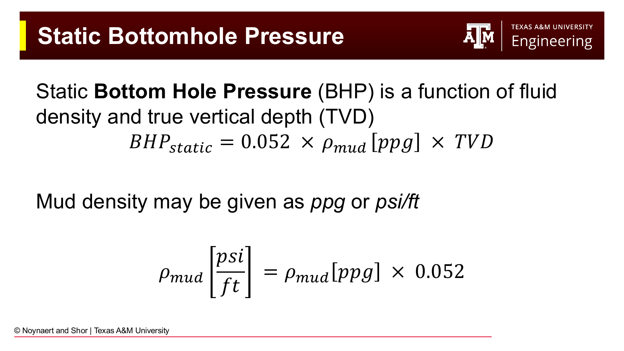
Fig. 79 The static bottomhole pressure equation — the foundation of all wellbore pressure calculations. Mud density in lb/gal multiplied by true vertical depth in feet and the conversion factor 0.052 gives pressure in psi.

Chapters 5 and 6 established how we measure and design the properties of drilling fluid. Now the question becomes: once that fluid is pumped down the drill string and back up the annulus, what pressures does it exert at every point in the wellbore?

Three practical questions motivate drilling hydraulics:

1. Downhole pressures. The bottomhole pressure during drilling, which includes both the static hydrostatic head and the friction generated by flowing mud, determines whether we are overbalanced (mud pressure exceeds pore pressure, which prevents a kick) and whether we are below the fracture gradient (which prevents lost circulation). Every foot drilled is governed by these twin constraints.

2. Drilling issues. Hole cleaning, the ability of the circulating mud to lift cuttings from the bit face to the surface, depends directly on annular velocity. Stuck pipe, pack-offs, and cuttings accumulation are all hydraulics problems.

3. Surface equipment selection. Before spudding a well, the drilling engineer calculates the total circulating pressure the system will require. The mud pumps must be rated to deliver that pressure at the planned flow rate. Getting this wrong means the well cannot be drilled as designed.

The calculation procedure developed in this chapter applies equally to the design phase (before the well is drilled) and to the operational phase (real-time interpretation of standpipe pressure while drilling).

---

7.2 The Wellbore Pressure System

7.2.1 Static Bottomhole Pressure

In the absence of fluid movement, the pressure at any depth in the wellbore is determined solely by the hydrostatic column of fluid above it:

\[\boxed{BHP_{static} = 0.052 \times \rho_{mud} \text{ (ppg)} \times TVD \text{ (ft)}}\]

Key Term: TVD vs. Measured Depth

True vertical depth (TVD) is the vertical distance from surface (the wellhead or the rig floor) to the point of interest: the component of depth that acts in the direction of gravity. Measured depth (MD) is the total length of the wellbore path, which is longer than TVD in a deviated well. Hydrostatic pressure depends only on TVD, not on MD. A 14,000 ft measured-depth well with a TVD of 10,000 ft has the same bottomhole pressure as a vertical 10,000 ft well, if both are full of the same weight mud.

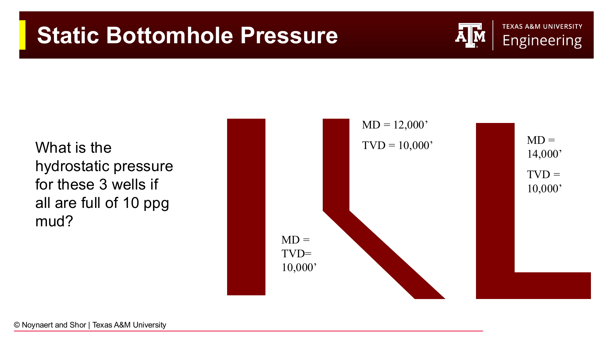
Fig. 80 Three wells with different trajectories but the same TVD (10,000 ft) all have the same hydrostatic bottomhole pressure if filled with the same mud weight. Only TVD matters for pressure.

7.2.2 Hydrostatics in Complex Fluid Columns

When the wellbore contains sections of different fluid densities, as during cementing operations, when spotting pills, or in completion and workover operations, the total bottomhole pressure is the sum of contributions from each fluid segment:

\[BHP = 0.052 \sum_i \rho_i \Delta L_i\]

where \(\rho_i\) is the density of fluid segment \(i\) and \(\Delta L_i\) is the ** vertical length** (not the actual depth) of that segment.

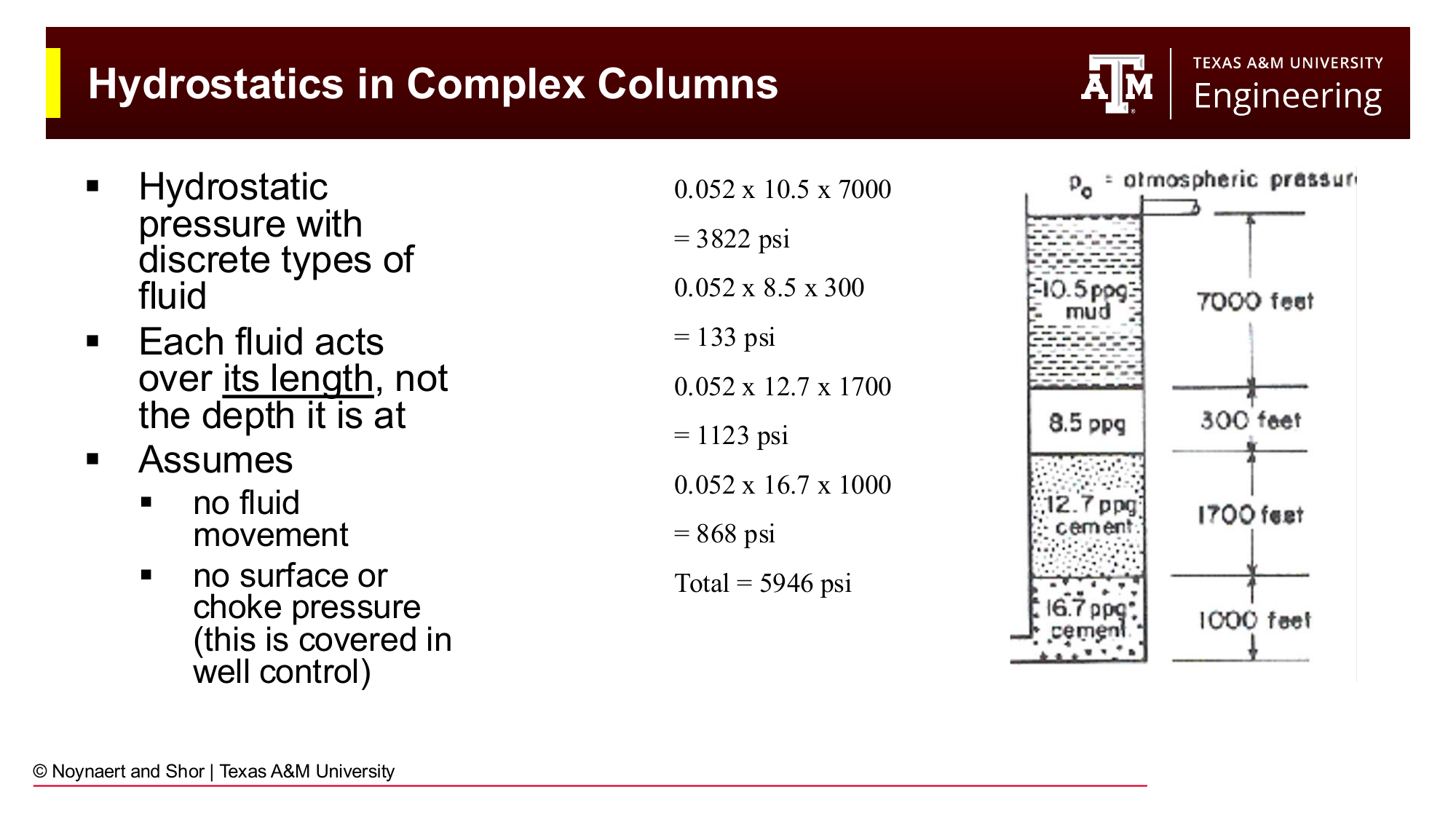
Fig. 81 Hydrostatic pressure in a complex fluid column. Each fluid acts over its own length, not over the total depth. The total BHP (5,946 psi) is the sum of the four segment contributions.

The key point, which catches students and experienced engineers alike, is that each fluid acts over its own vertical length, not over the depth it sits at. For example, a 1,000 ft tail of 16.7 ppg cement at the bottom of a 10,000 ft well contributes \(0.052 \times 16.7 \times 1000 = 868\) psi, not \(0.052 \times 16.7 \times 10{,}000\).

7.2.3 Equivalent Circulating Density (ECD)

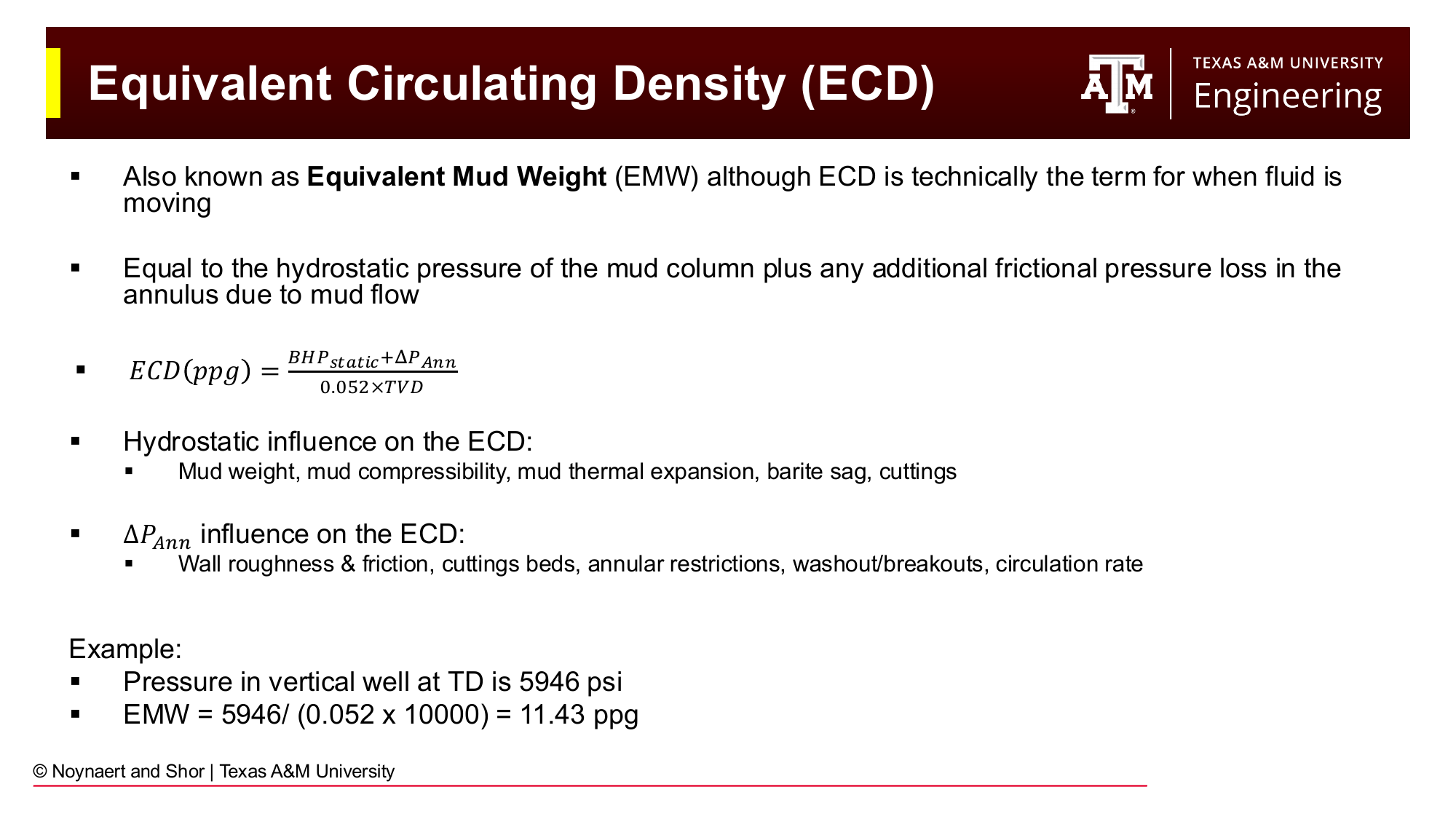
Fig. 82 ECD (equivalent circulating density) equals the hydrostatic pressure plus the annular frictional pressure loss, all expressed as an equivalent mud weight in ppg. ECD is always greater than the static mud weight.

When mud is circulating, friction between the flowing fluid and the wellbore wall adds pressure to the annular side of the system. The equivalent circulating density (ECD) expresses the total bottomhole pressure: the hydrostatic pressure plus annular friction, as a mud weight:

\[\boxed{ECD \text{ (ppg)} = \rho_{mud} + \frac{\Delta P_{Ann} \text{ (psi)}}{0.052 \times TVD \text{ (ft)}}}\]

When flowing, ECD is always higher than the static mud weight. This means that circulating mud exerts more pressure on the formation than the same mud at rest. In wells with a narrow drilling window, where pore pressure and fracture gradient are close together, ECD management is as important as mud weight selection.

Factors that increase ECD include: higher mud weight, higher viscosity, higher flow rate, smaller annular clearances, cuttings loading in the annulus, and wellbore roughness. Factors that decrease ECD include: lower flow rate, larger annular clearance, and lighter or less viscous mud.

---

7.3 BHA Components and Geometry

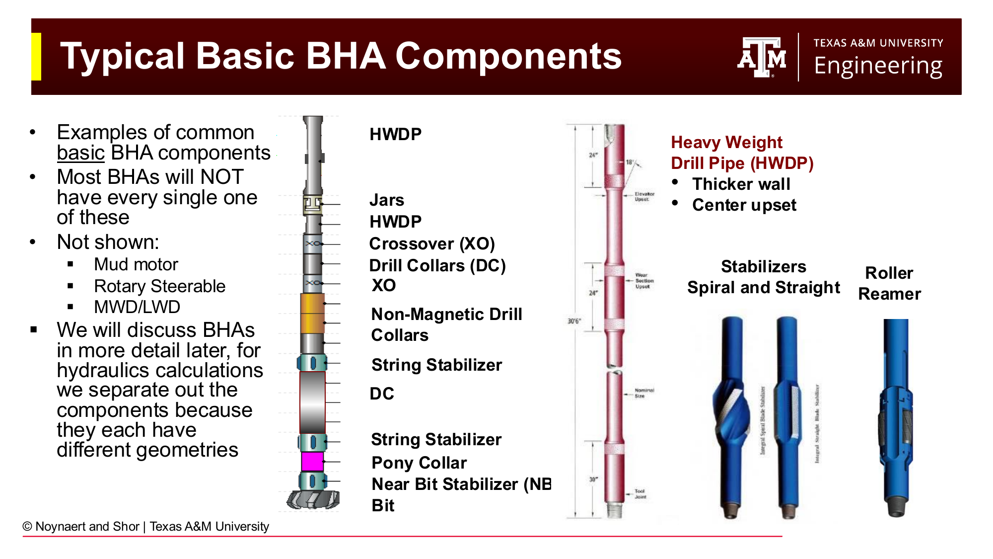
Fig. 83 Typical basic BHA components from top to bottom: HWDP, jars, crossover subs, drill collars, stabilizers, roller reamer, non-magnetic drill collars, pony collar, near-bit stabilizer, and bit. Each component has a different internal diameter (ID) and external diameter (OD), creating a new geometry segment for pressure loss calculations.

The bottom hole assembly (BHA) is the lower portion of the drill string, extending from the bit up through the drill collars and into the transition to drill pipe. Each component of the BHA has a distinct internal diameter (the flow passage) and external diameter (which defines the annular gap between the component and the wellbore wall).

Every time the geometry changes, a new pressure loss segment begins. This is the fundamental principle of hydraulics calculations: the flow path is divided into segments of constant geometry, and the pressure loss is calculated separately for each segment. Typical geometry change points include:

• Transition from drill pipe to HWDP

• Transition from HWDP to drill collars

• Transition from one drill collar size to another

• Locations of stabilizers or reamers

• Transition from cased hole to open hole (changes the outer boundary of the annulus)

• The bit nozzles (the largest single pressure drop in the system)

Draw a Picture

Before doing any pressure loss calculation, draw a schematic of the wellbore showing every geometry segment. Label the inside diameter (ID) of each component of the drill string, the outside diameter (OD) of each component, the diameter of the wellbore (or casing ID) for each section, and the length of each. Once the picture is drawn and the geometry is organized, the calculation becomes straightforward: pick a model, apply it to each segment, and add up the results.

This is the single most effective step to avoid errors in hydraulics calculations. A student who draws the picture almost always gets the problem right; one who doesn’t often makes errors in the segment boundaries.

7.3.1 Mud Motors (PDMs)

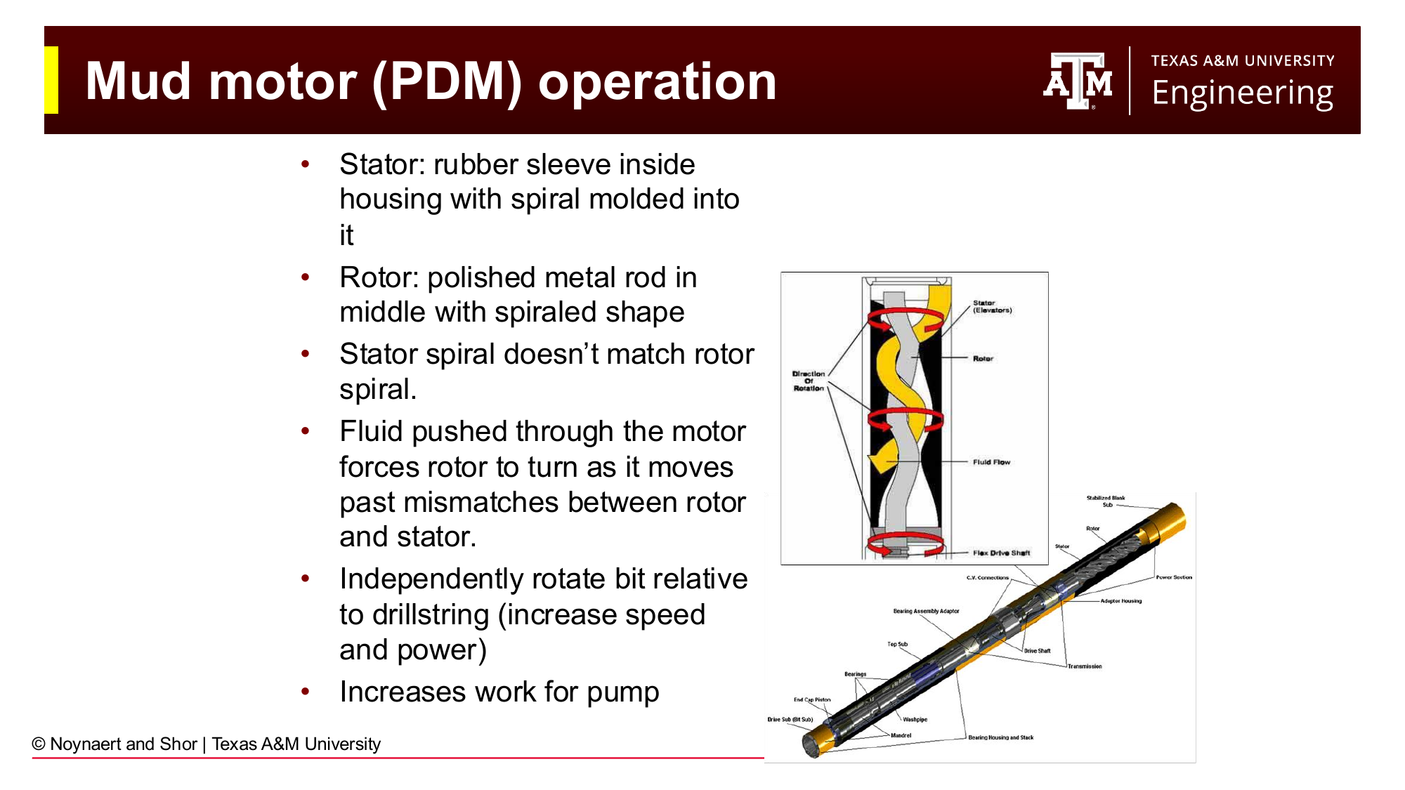
Fig. 84 A positive displacement mud motor (PDM) converts hydraulic energy from flowing mud into mechanical rotation of the bit. The rotor-stator mismatch forces the rotor to turn as fluid passes through. Mud motors represent a significant pressure restriction in the drill string and must be accounted for in hydraulics calculations.

A positive displacement mud motor (PDM), is a common BHA component in directional drilling. Fluid pumped through the motor causes a spiral rotor to turn inside a stationary rubber stator, converting hydraulic energy to mechanical rotation that drives the bit. This allows the bit to rotate even when the entire drill string is not being rotated, and is useful for directional steering.

From a hydraulics standpoint, the mud motor is a large restriction in the drill string. The pressure drop across the motor \(\Delta P_{motor}\) can be 200–800 psi or more, depending on the motor size, flow rate, and torque output. This must be included in the standpipe pressure calculation. Vendor-specific charts or the general power relationship are used to estimate \(\Delta P_{motor}\).

---

7.4 The Standpipe Pressure Equation

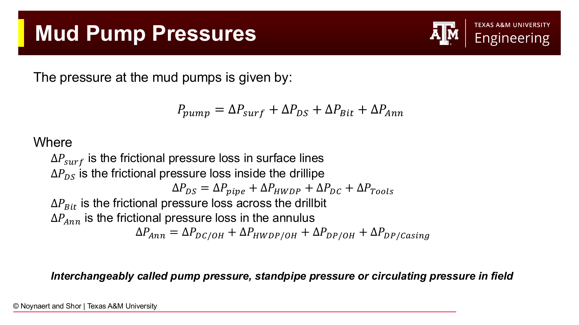
Fig. 85 Standpipe pressure (SPP) is the sum of all frictional pressure losses in the circulating system: surface lines, drill pipe, HWDP, drill collars, tools (including mud motor), bit nozzles, and the annulus segments.

The total pressure at the mud pumps, called the standpipe pressure (SPP) or circulating pressure, is the sum of all frictional pressure losses in the circulating system:

\[P_{pump} = \Delta P_{surf} + \Delta P_{DS} + \Delta P_{Bit} + \Delta P_{Ann}\]

where:

• \(\Delta P_{surf}\) = frictional loss in surface lines (standpipe, rotary hose, swivel, kelly or top drive)

• \(\Delta P_{DS}\) = frictional loss inside the drill string = \(\Delta P_{pipe} + \Delta P_{HWDP} + \Delta P_{DC} + \Delta P_{Tools}\)

• \(\Delta P_{Bit}\) = pressure drop across the bit nozzles

• \(\Delta P_{Ann}\) = frictional loss in the annulus = \(\Delta P_{DC/OH} + \Delta P_{HWDP/OH} + \Delta P_{DP/OH} + \Delta P_{DP/Csg}\)

7.4.1 Path Dependency and the “Gauge” Concept

The key to applying this equation correctly is understanding that pressure calculations are path dependent. You must know where your (real or hypothetical) pressure gauge is, and then account only for the pressure contributions downstream of that gauge — the segments that the fluid will pass through after leaving the gauge.

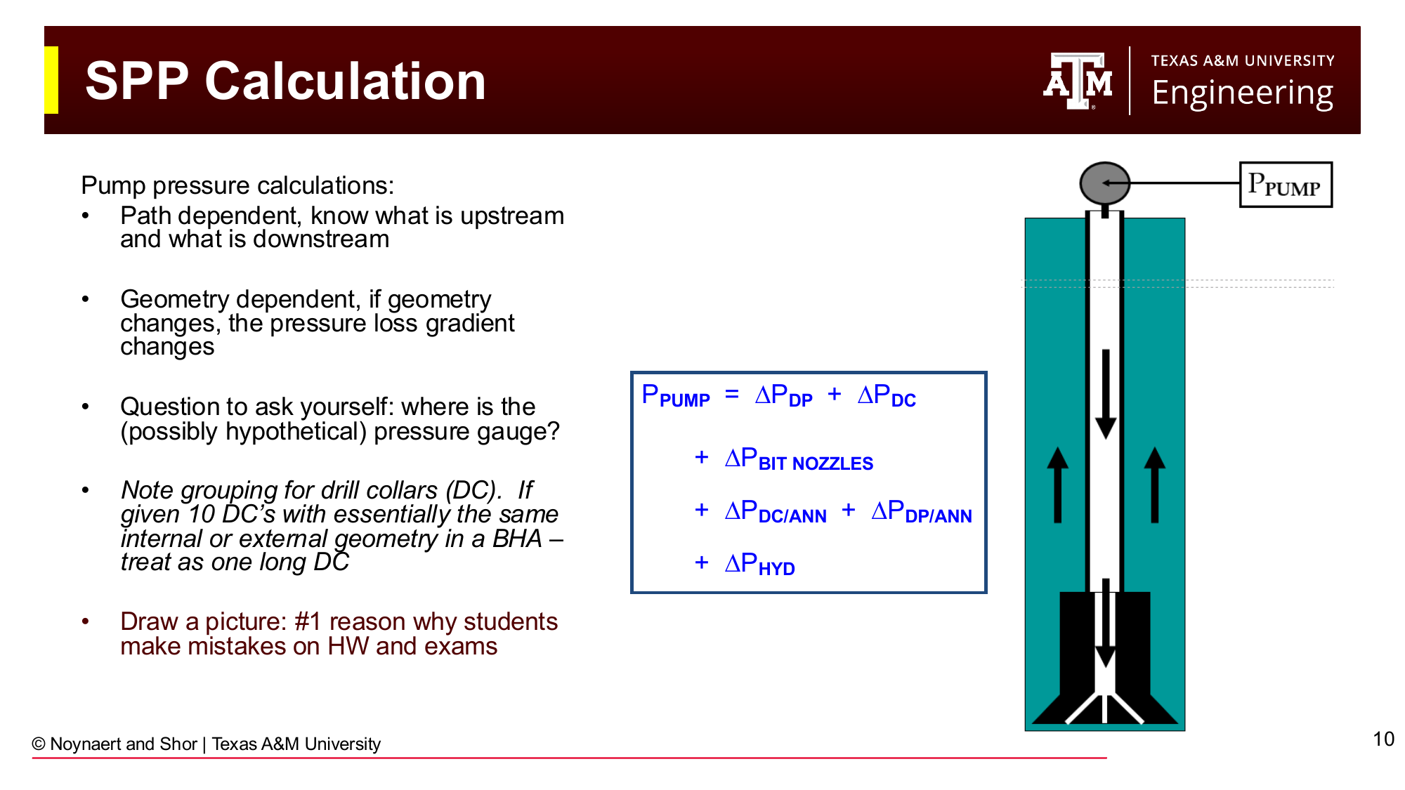
Fig. 86 Identifying upstream and downstream segments for a standpipe pressure calculation. All segments downstream of the pump (the gauge) contribute to SPP. When calculating bottomhole pressure, the drill string interior is upstream of the bottomhole point and does not contribute.

For standpipe pressure: the gauge is at the pump. Everything downstream contributes: surface lines, drill string interior, bit, and annulus.

For bottomhole pressure: the gauge is at the bit. Everything downstream of the bit contributes: all annular segments. The entire drill string interior is upstream: it is not counted. The frictional pressure in the drill pipe interior was already “spent” getting the fluid down to the bit; that energy does not add to the BHP as seen from the formation. The same applies to the drillbit.

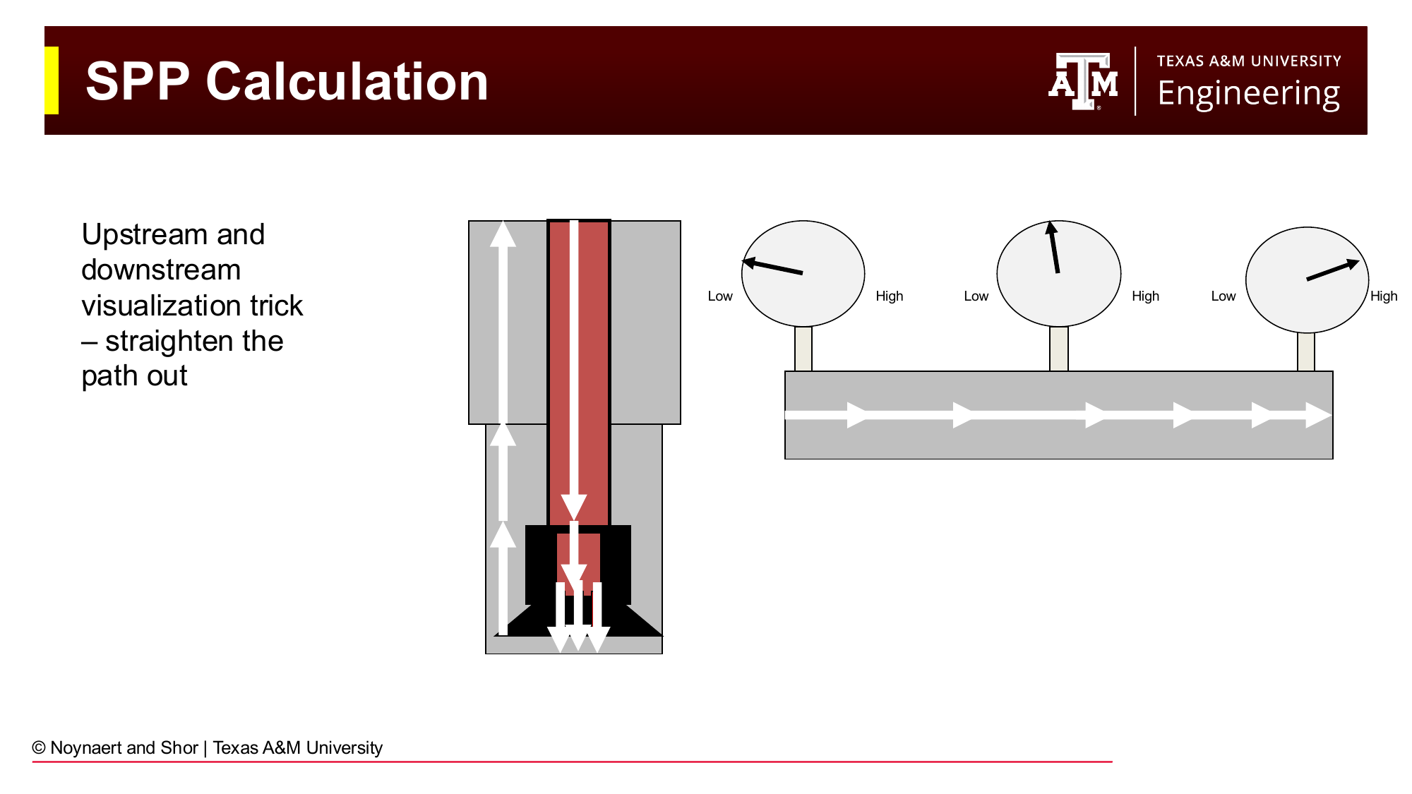
Fig. 87 Visualizing the circulating system by “straightening out” the flow path. Fluid flows from low pressure (surface) to high pressure (pump) on the intake side, and from high pressure (pump) to progressively lower pressure as it travels down the drill string, through the bit, and up the annulus. Each segment adds a pressure drop.

A useful mental model: straighten out the flow path so it looks like a single pipe with segments side by side. Pressure increases from zero (at the mud pit outlet) to maximum (at the pump suction), decreases as you move down the drill string, drops sharply at the bit, and then decreases further as you move up the annulus.

---

7.5 Five-Step Calculation Procedure

Calculating frictional pressure loss in any segment follows the same five steps, applied to each segment separately:

1. Select the appropriate fluid rheological model

2. Calculate fluid velocity in the segment

3. Calculate the Reynolds number and determine flow regime

4. Calculate the friction factor

5. Calculate the frictional pressure loss

Step 1: Select the Fluid Model

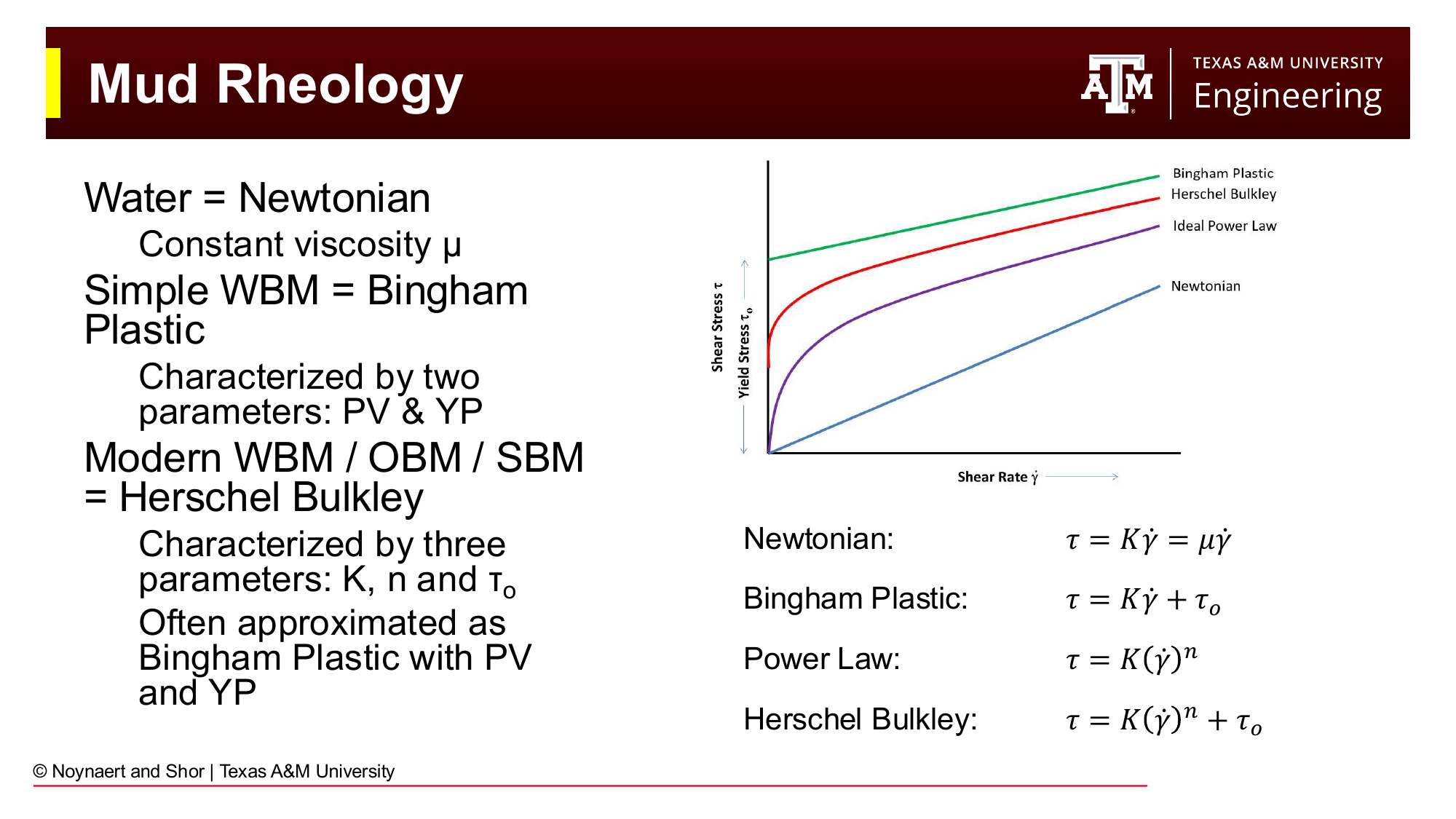
Fig. 88 The four rheological models and their associated drilling fluid types. Herschel-Bulkley is the most accurate general model. Bingham Plastic is widely used in field practice for its simplicity.

As established in Chapters 5 and 6, the four models are:

Model	Equation	Parameters	Typical Application
Newtonian	\(\tau = \mu\dot{\gamma}\)	\(\mu\)	Fresh water, thin brines
Bingham Plastic	\(\tau = PV\dot{\gamma} + YP\)	PV, YP	Simple WBM; standard field reporting
Power Law	\(\tau = K\dot{\gamma}^n\)	\(K\), \(n\)	Intermediate complexity
Herschel-Bulkley	\(\tau = K\dot{\gamma}^n + \tau_0\)	\(K\), \(n\), \(\tau_0\)	Most modern WBM, OBM, SBM; API recommended

In practice: for quick field calculations, Bingham Plastic is most common. For wellbore design and detailed hydraulics programs, Herschel-Bulkley is preferred. Newtonian should only be used when the fluid truly has no yield stress (clean brines, fresh water).

Step 2: Calculate Fluid Velocity

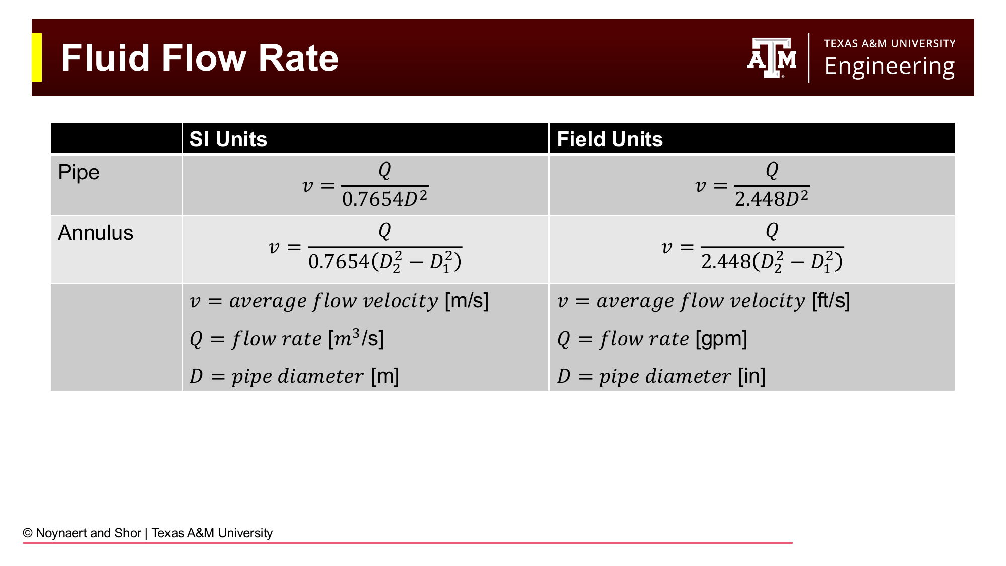
Fig. 89 Fluid velocity equations for pipe and annular flow in both SI and field units. Note that every geometry change requires a new velocity calculation, since flow rate is constant but geometry is not.

Flow rate \(Q\) (gpm (gal/min) in field units) is conserved around the circulating loop. Conservation of mass means what goes in must come out, unless a kick or a loss is occuring. In this chapter, we assume that the well is stable and a kick is not being taken. But velocity changes whenever the cross-sectional area changes.

In the drill string (pipe flow):

\[v \text{ (ft/s)} = \frac{Q \text{ (gpm)}}{2.448 \, D^2 \text{ (in}^2\text{)}}\]

In the annulus:

\[v_{ann} \text{ (ft/s)} = \frac{Q \text{ (gpm)}}{2.448 (D_2^2 - D_1^2) \text{ (in}^2\text{)}}\]

where \(D_2\) is the wellbore (or casing) inner diameter and \(D_1\) is the outer diameter of the drill string component.

Since geometry terms are squared in these expressions, a small change in diameter produces a significant change in velocity. A 25% increase in diameter reduces velocity by 56%. This propagates directly into the pressure loss calculation.

Step 3: Reynolds Number and Flow Regime

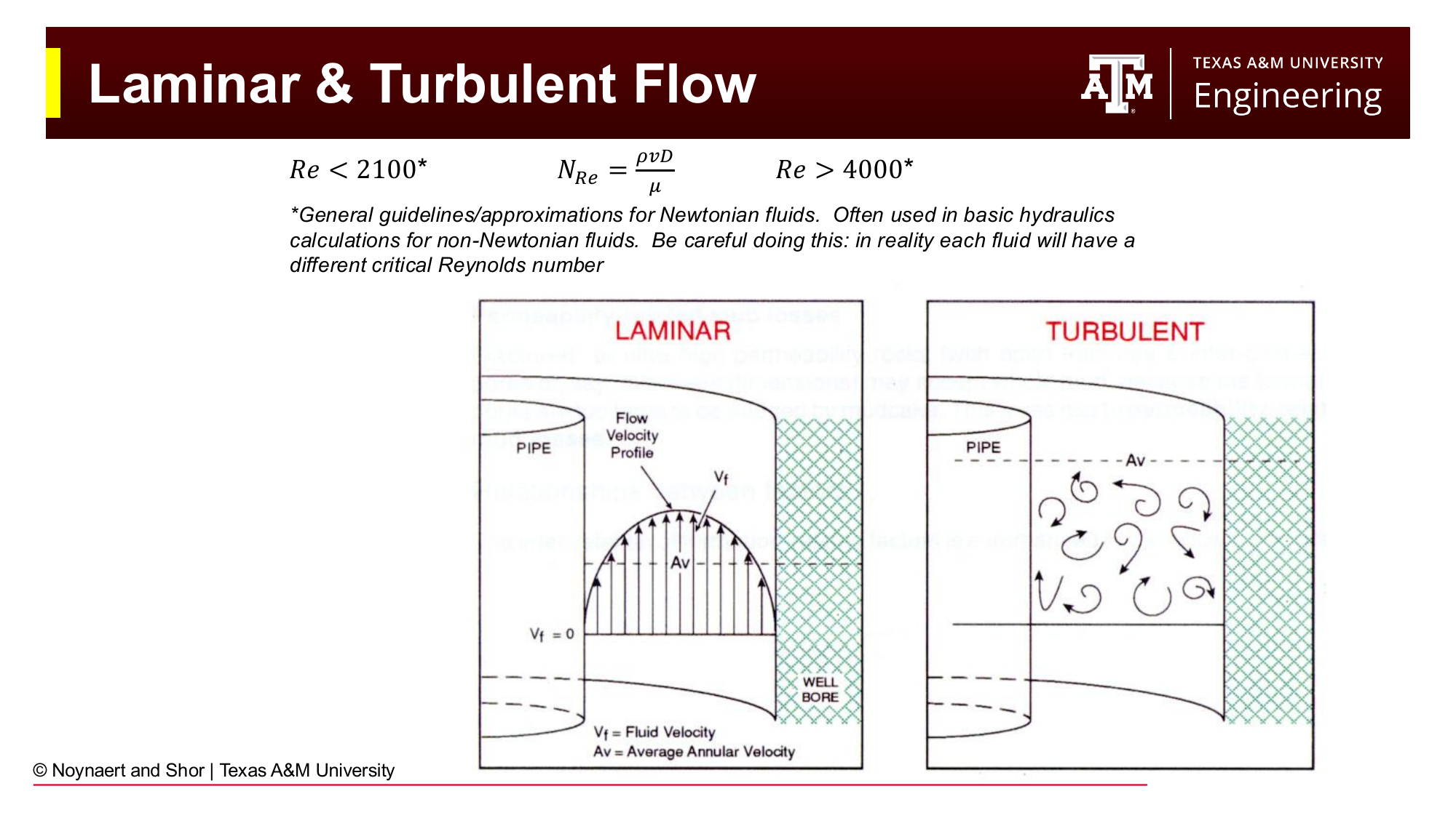
Fig. 90 Laminar flow (Re < 2100) has smooth, organized streamlines; turbulent flow (Re > 4000) has chaotic, mixing flow. The transition zone between these bounds is complex and is typically included in the turbulent regime for practical calculations.

The Reynolds number is a dimensionless ratio of inertial to viscous forces that determines whether the flow is laminar or turbulent:

\[N_{Re} = \frac{\rho v D}{\mu}\]

For practical purposes:

• \(N_{Re} < 2100\): laminar flow (viscous forces dominate; organized flow)

• \(2100 < N_{Re} < 4000\): transition (typically treated as turbulent in practice)

• \(N_{Re} > 4000\): turbulent flow (inertial forces dominate; chaotic mixing)

These thresholds were derived for Newtonian fluids. Non-Newtonian fluids (Bingham Plastic, Power Law, Herschel-Bulkley) have modified Reynolds number expressions that account for their yield stress and shear-thinning behavior. The key difference: Bingham Plastic and Herschel-Bulkley fluids have an apparent viscosity that depends on the local shear rate, so the Reynolds number must be expressed in terms of an effective (apparent) viscosity.

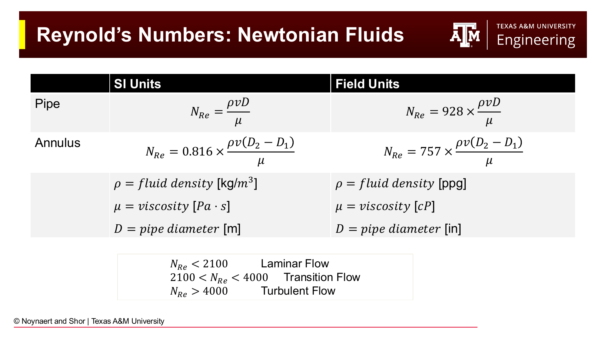
Fig. 91 Reynolds number equations for Newtonian fluids in pipe and annular geometry, in both SI and field units. For non-Newtonian fluids, the viscosity term is replaced by an apparent viscosity that depends on local shear rate.

Newtonian (field units):

\[N_{Re,pipe} = 928 \frac{\rho v D}{\mu} \qquad N_{Re,ann} = 757 \frac{\rho v (D_2 - D_1)}{\mu}\]

Bingham Plastic: An apparent viscosity \(\mu_a\) is calculated that accounts for both PV and YP at the given flow velocity, then used in the standard Reynolds number equation:

\[\mu_{a,pipe} = PV + \frac{6.66 \cdot YP \cdot D}{v} \qquad \mu_{a,ann} = PV + \frac{5 \cdot YP \cdot (D_2 - D_1)}{v}\]

\[N_{Re} = 928 \frac{\rho v D}{\mu_a} \quad (\text{pipe}) \qquad N_{Re} = 757 \frac{\rho v (D_2-D_1)}{\mu_a} \quad (\text{annulus})\]

Power Law: The critical Reynolds number for transition to turbulence depends on the flow behavior index \(n\):

\[N_{Re,crit,lam} = 3470 - 1370n \qquad N_{Re,crit,turb} = 4270 - 1370n\]

Herschel-Bulkley: The most complete model; Reynolds number and critical Reynolds number expressions are more involved and best implemented in a spreadsheet..

Step 4: Friction Factor

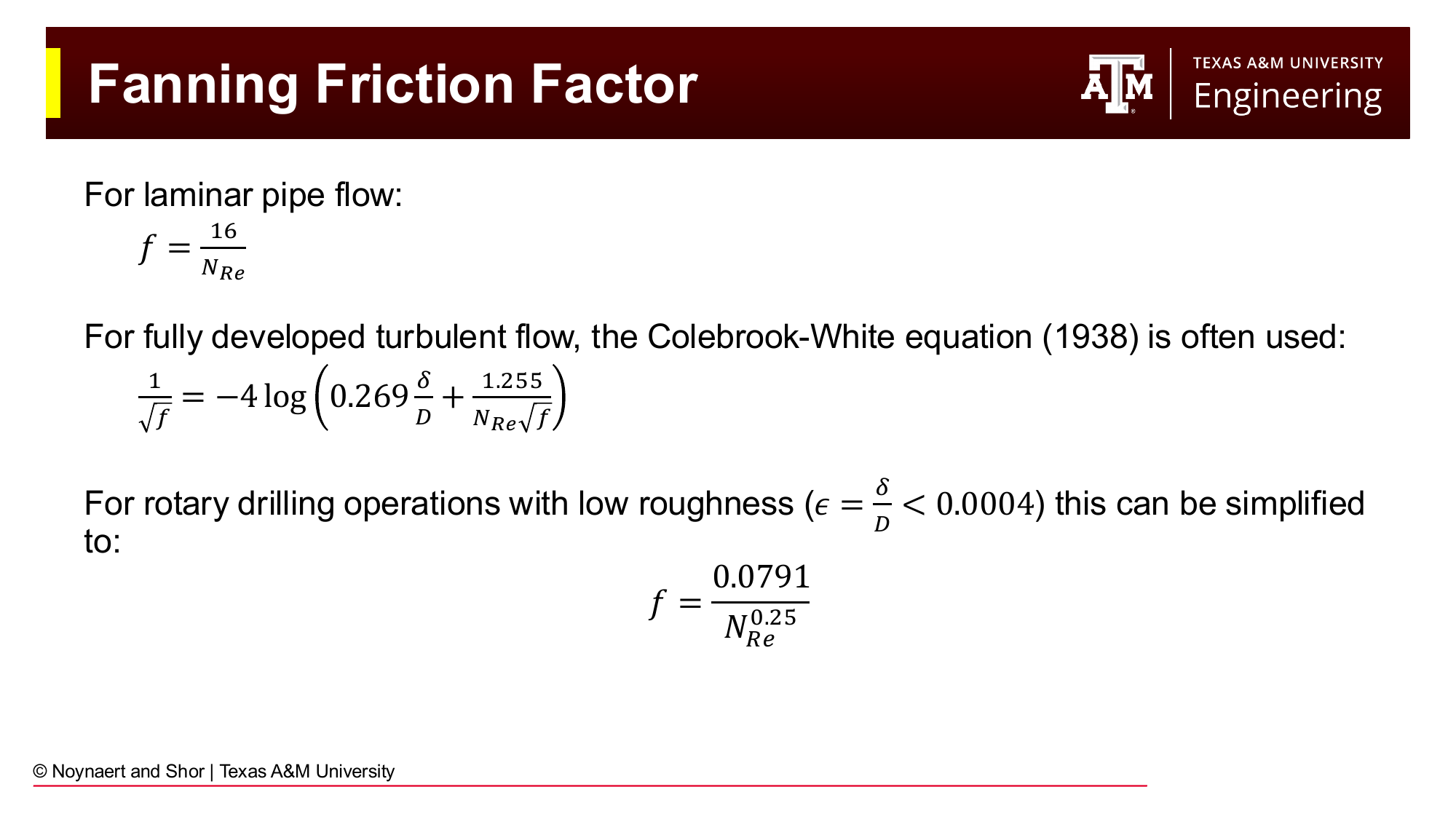
Fig. 92 Fanning friction factor equations for laminar and turbulent flow. For laminar flow, \(f = 16/Re\). For turbulent flow in smooth pipe, the simplified Colebrook expression gives \(f = 0.0791/Re^{0.25}\). The full Colebrook-White equation accounts for pipe roughness.

The Fanning friction factor \(f\) is a dimensionless measure of the ratio of wall shear stress to the kinetic energy of the fluid:

Laminar flow:

\[f = \frac{16}{N_{Re}}\]

Turbulent flow in smooth or low-roughness pipe (typical for drill pipe and drill collars):

\[f = \frac{0.0791}{N_{Re}^{0.25}}\]

For turbulent flow with significant pipe roughness, the full Colebrook-White equation is used:

\[\frac{1}{\sqrt{f}} = -4\log\left(0.269\frac{\delta}{D} + \frac{1.255}{N_{Re}\sqrt{f}}\right)\]

where \(\delta\) is the absolute pipe roughness. For commercial steel drill pipe (\(\delta \approx 0.000013\) in), the smooth-pipe approximation is adequate for most drilling calculations.

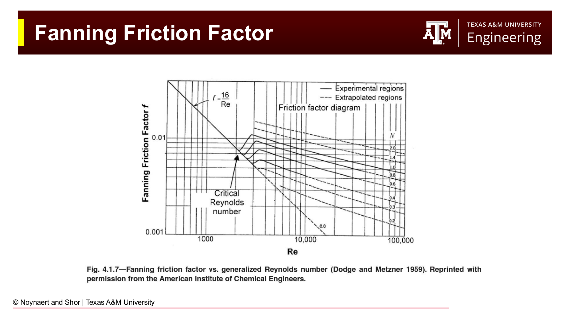
Fig. 93 The Moody chart (Fanning friction factor vs. Reynolds number). For laminar flow, \(f = 16/Re\) regardless of roughness. For turbulent flow, the friction factor depends on both Reynolds number and relative roughness. The smooth-pipe approximation (\(f = 0.0791/Re^{0.25}\)) is adequate for most drilling calculations.

Note, for calculations with Newtonian fluids, an explicit calculations for friciton factor is not needed.

Step 5: Frictional Pressure Loss

The Fanning equation gives the frictional pressure gradient (psi/ft):

Field units: $\(\frac{dP}{dL} = \frac{f \rho_f v^2}{25.8 D}\)$

To get total pressure loss in a segment of length \(\Delta L\): \(\Delta P_f = (dP/dL) \times \Delta L\).

Alternatively, simplified expressions are used for each model and flow regime.

Newtonian fluids:

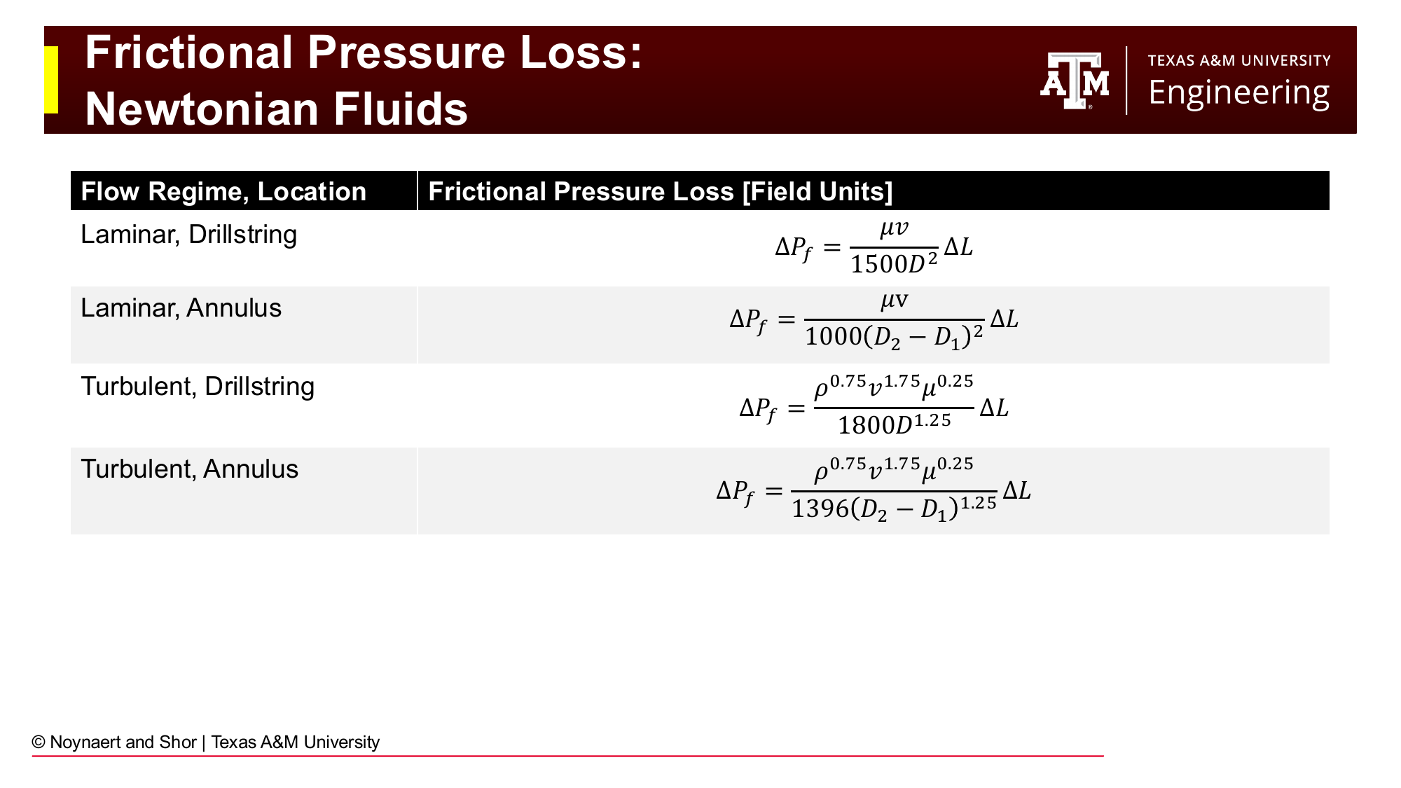
Fig. 94 Frictional pressure loss equations for Newtonian fluids in laminar and turbulent flow, for both pipe and annular geometry. All equations are in field units.

Flow regime	Location	\(\Delta P_f\) (psi)
Laminar	Drillstring	\(\dfrac{\mu v}{1500 D^2} \Delta L\)
Laminar	Annulus	\(\dfrac{\mu v}{1000 (D_2-D_1)^2} \Delta L\)
Turbulent	Drillstring	\(\dfrac{\rho^{0.75} v^{1.75} \mu^{0.25}}{1800 D^{1.25}} \Delta L\)
Turbulent	Annulus	\(\dfrac{\rho^{0.75} v^{1.75} \mu^{0.25}}{1396 (D_2-D_1)^{1.25}} \Delta L\)

Bingham Plastic fluids:

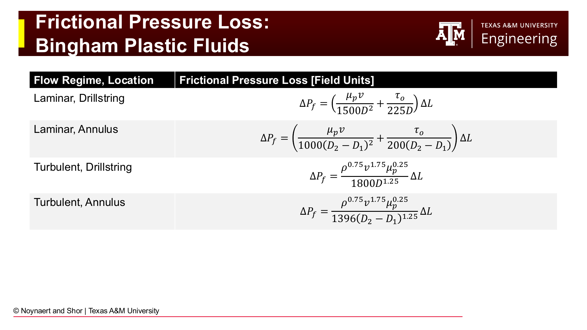
Fig. 95 Frictional pressure loss equations for Bingham Plastic fluids. The laminar expressions include a yield-point term (YP/D or YP/(D₂-D₁)); the turbulent expressions are the same as Newtonian but use PV in place of viscosity.

Flow regime	Location	\(\Delta P_f\) (psi)
Laminar	Drillstring	\(\left(\dfrac{PV \cdot v}{1500 D^2} + \dfrac{YP}{225 D}\right) \Delta L\)
Laminar	Annulus	\(\left(\dfrac{PV \cdot v}{1000 (D_2-D_1)^2} + \dfrac{YP}{200 (D_2-D_1)}\right) \Delta L\)
Turbulent	Drillstring	\(\dfrac{\rho^{0.75} v^{1.75} PV^{0.25}}{1800 D^{1.25}} \Delta L\)
Turbulent	Annulus	\(\dfrac{\rho^{0.75} v^{1.75} PV^{0.25}}{1396 (D_2-D_1)^{1.25}} \Delta L\)

The yield point appears in the laminar expressions because, in laminar flow, the YP directly contributes to the pressure gradient required to keep the fluid moving. In turbulent flow, the YP effect is much less significant compared to viscous and inertial forces.

---

7.6 Bit Pressure Loss

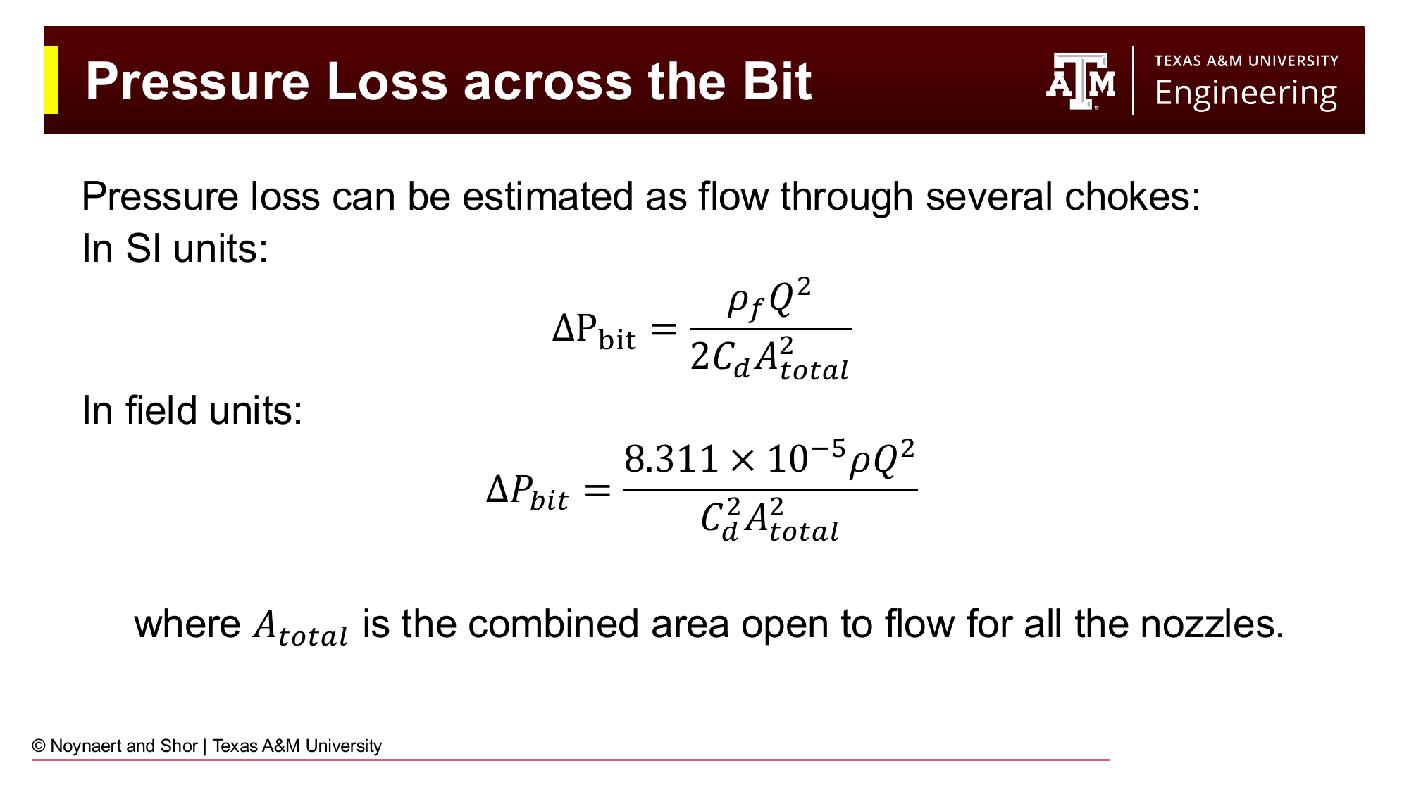
Fig. 96 Pressure loss at the bit nozzles. The bit is equivalent to flow through a set of orifice chokes. The pressure drop is proportional to \(\rho Q^2\) and inversely proportional to the square of the total nozzle area.

The drill bit nozzles are deliberately sized small to create a high-velocity fluid jet at the bit face. This jet performs several functions: it cleans cuttings from the bit face, cools the cutting elements, and creates a hydraulic impact force at the formation. As a result, the pressure drop across the nozzles is typically the largest single pressure drop in the circulating system — often as high as 1,000–2,500 psi.

The bit pressure drop is modeled as flow through parallel orifice chokes:

\[\Delta P_{bit} = \frac{8.311 \times 10^{-5} \rho Q^2}{C_d^2 A_{total}^2}\]

where:

• \(\rho\) = mud density (ppg)

• \(Q\) = flow rate (gpm)

• \(C_d\) = discharge coefficient (~0.95 for jets, 0.8 for open-face bits)

• \(A_{total}\) = total nozzle area (in²) = sum of areas of all nozzles

Nozzle sizes are specified in 32nds of an inch. A “12” nozzle has a diameter of 12/32 = 0.375 in, with an area of \(\pi(0.375/2)^2 = 0.110\) in². Three 12-nozzle bits would have \(A_{total} = 3 \times 0.110 = 0.330\) in².

---

7.7 Mud Motor Pressure Drop

When a mud motor is in the BHA, it represents an additional hydraulic restriction. The pressure drop through the motor can be estimated from the horsepower relationship:

\[HP_{motor} = \frac{\eta \Delta p_{motor} Q}{1714}\]

\[T = 5252 \frac{HP_{motor}}{N}\]

where \(\eta\) is motor efficiency (~0.8–0.9), \(\Delta p_{motor}\) is the pressure drop across the motor (psi), \(Q\) is flow rate (gpm), \(N\) is rotational speed of the bit (rpm), and \(T\) is torque (ft-lb). In practice, the motor manufacturer provides differential pressure vs. flow rate charts for their specific tool.

---

7.8 Eccentric Annuli

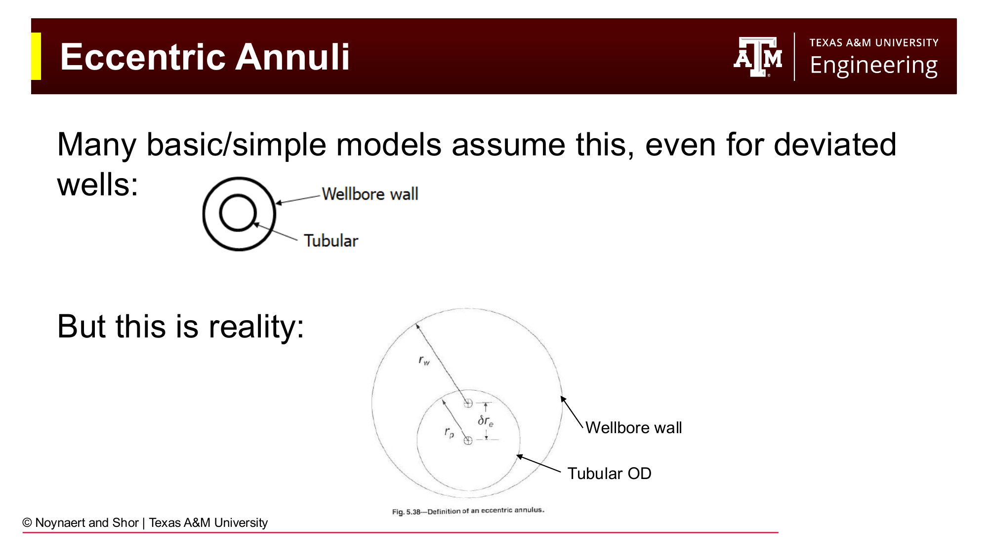
Fig. 97 Left: concentric annulus assumed by most simple models. Right: eccentric annulus (drill pipe lying on the low side of a deviated wellbore), which is the actual condition in most deviated wells. The fluid preferentially flows through the larger gap, reducing the effective pressure loss.

All the pressure loss equations above assume the drill string is concentric inside the wellbore: the drill pipe is centered, with equal clearance on all sides. In reality, particularly in deviated wells, the drill string lies on the low side of the wellbore under gravity, creating an eccentric geometry: a large gap above the pipe, a small or zero gap below.

Eccentric geometry reduces annular frictional pressure loss below the concentric prediction because the fluid preferentially flows through the larger gap. A correction factor \(C_e\) (Haciislamoglu and Langlinais, 1990) can be applied to the concentric pressure gradient:

\[\left(\frac{dP}{dL}\right)_{eccentric} = C_e \times \left(\frac{dP}{dL}\right)_{concentric}\]

where \(C_e < 1\) for any eccentricity \(> 0\).

For wellbore cleaning purposes, eccentricity is actually a problem: the small gap on the low side sees very low velocity, and cuttings beds accumulate there. This is a primary driver of poor hole cleaning in horizontal wells.

---

7.9 Bringing It All Together: Standpipe Pressure

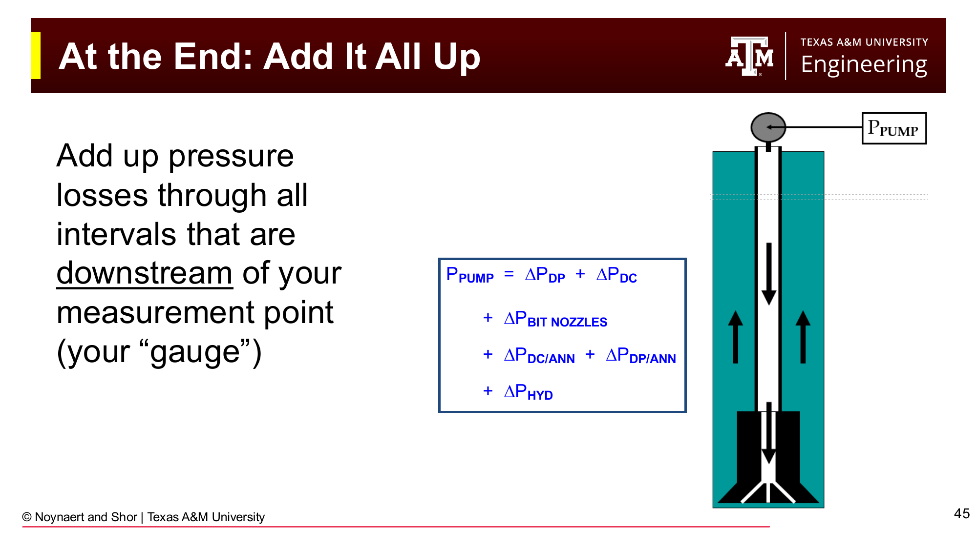
Fig. 98 Standpipe pressure is the sum of all downstream pressure losses: drill pipe interior, drill collar interior, bit nozzles, drill collar/open-hole annulus, drill pipe/open-hole annulus, and the hydrostatic difference between the drill string and annular columns.

Having calculated the pressure loss in each segment, the total pump pressure is assembled by summation:

\[P_{pump} = \Delta P_{DP} + \Delta P_{DC} + \Delta P_{Bit} + \Delta P_{DC/OH} + \Delta P_{DP/OH} + \Delta P_{DP/Csg} + \Delta P_{hyd}\]

The hydrostatic term \(\Delta P_{hyd}\) accounts for the fact that in most wells, the mud in the drill string and the mud in the annulus are at the same density, so their hydrostatic contributions cancel. However, during cementing, tripping with different densities on each side, or in any operation where drillstring and annular fluid densities differ, this term is non-zero.

---

7.10 Pump Output Calculations

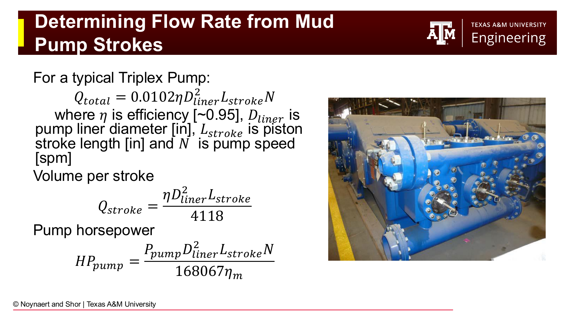
Fig. 99 Triplex pump output calculations. Volume per stroke is a function of liner diameter and stroke length; total flow rate depends also on pump speed (strokes per minute). These calculations are essential for lag time estimation in well control operations.

Knowing how many pump strokes it takes to move fluid from one point in the well to another is critical for well control (discussed in Chapter 8). A triplex pump (three cylinders) outputs:

\[Q_{total} \text{ (gpm)} = 0.0102 \, \eta \, D_{liner}^2 \, L_{stroke} \, N\]

where \(\eta\) is volumetric efficiency (~0.95), \(D_{liner}\) is the liner (piston) diameter (in), \(L_{stroke}\) is the stroke length (in), and \(N\) is the pump speed (spm = strokes per minute).

Volume per stroke:

\[Q_{stroke} \text{ (bbl/stroke)} = \frac{\eta D_{liner}^2 L_{stroke}}{4118}\]

The lag time, the number of strokes to move fluid from the bit to surface through the annulus, is simply the annular volume (bbl) divided by \(Q_{stroke}\) (bbl/stroke). This tells the driller exactly how many strokes after a density change at the pump it will be before the new fluid reaches the surface: critical for monitoring for kicks and for understanding bottomhole conditions.

---

7.11 Calculation to Reality: Field Considerations

The equations in this chapter assume ideal conditions: a perfectly known geometry, uniform fluid properties throughout the wellbore, and stable conditions. In practice, none of these assumptions hold exactly, and the calculated standpipe pressure will differ from the observed SPP by some amount.

Sources of uncertainty:

Fluid properties change between the surface mud check and the downhole condition. Temperature and pressure alter viscosity and density (as discussed in Chapter 6). The last mud check may have been hours ago.

Geometry is not perfectly known. Drill pipe ID is measured when new; an old pipe may have been worn or damaged. Hole size is nominal — the actual wellbore may be washed out by several inches in soft formations. Geometry enters the pressure loss equations to the second power: a quarter-inch enlargement in an 8.75-inch hole reduces the \(D_2^2 - D_1^2\) term by about 6%, and the velocity — which also enters squared — is likewise affected.

What to do when calculated and observed SPP don’t match:

First, verify that all input data is current and correct. Recalibrate geometry assumptions, starting with hole size (the most uncertain parameter). Get a fresh mud check. If a correction factor must be applied, do so transparently and note that consistent large corrections point to bad inputs, not bad equations.

Empirical correction factors: A power-law fit to measured SPP vs. flow rate data can be used to calibrate the calculation to field observations:

\[\Delta P_{fric} = c \cdot Q^m\]

A field engineer may fit this model by pumping at two different flow rates \(Q_1\) and \(Q_2\) while off bottom and recording surface pump pressure \(SPP_1\) and \(SPP_2\). If the bit is off bottom, SPP is approximately equal to the fricitonal pressure loss in the entire system. \(c\) and \(m\) may be fit using:

\[m = \frac{\log\left(\frac{SPP_1}{SPP_2}\right)}{\log\left(\frac{Q_1}{Q_2}\right)}\]

and

\[c = \frac{SPP_1}{Q_1^m} = \frac{SPP_2}{Q_2^m}\]

Note, this approximation will only be valid for values of Q near \(Q_1\) and \(Q_2\).

---

7.12 ECD and the Drilling Window

Fig. 100 Factors that increase or decrease ECD during various wellbore operations (drilling, tripping in hole, tripping out of hole, running casing). Understanding how operational activities shift the effective bottomhole pressure is essential for staying within the drilling window.

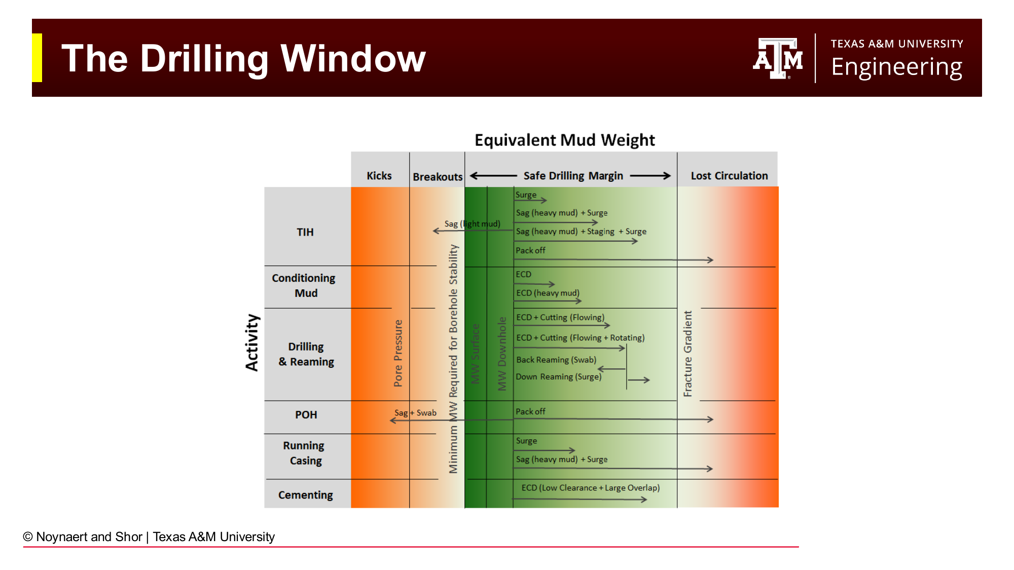
Fig. 101 The drilling window showing pore pressure gradient, fracture gradient, and the equivalent mud weight (or ECD) during different operations. Trip margins ensure the wellbore remains overbalanced during tripping. Swab and surge pressures represent transient excursions of the ECD outside its steady-state circulating value.

The drilling window from Chapter 2 now takes on its full quantitative meaning: the mud weight must be selected so that the static hydrostatic pressure exceeds pore pressure at all times, and the ECD (during circulating) remains below the fracture gradient. In addition:

• Surge pressure (tripping in hole): the annulus is displaced by the incoming drill string, temporarily increasing BHP. Running in hole too fast in tight wells can fracture the formation.

• Swab pressure (tripping out of hole): the drill string acts like a piston pulling upward, temporarily decreasing BHP. Pulling out too fast in high-pore-pressure zones can induce a kick.

Trip margins of 0.5 ppg are commonly maintained to provide a buffer between the static mud weight and both the pore pressure gradient (below) and the fracture gradient (above).

---

Worked Examples

Example 7.1 — Standpipe Pressure Calculation (Bingham Plastic, Laminar Flow)

Problem: A well is drilled with the following configuration:

• Mud: 11.5 ppg, PV = 25 cP, YP = 14 lb/100 ft²

• Drill pipe: OD = 5.0 in, ID = 4.276 in; length = 9,800 ft

• Drill collars: OD = 6.75 in, ID = 2.875 in; length = 500 ft

• Open-hole diameter: 8.75 in (drill collar section and drill pipe section same hole size)

• Bit: three nozzles, each 13/32 in

• Flow rate: 400 gpm

• TVD = 10,300 ft (vertical well)

Calculate the standpipe pressure.

Solution:

Step 1: Calculate velocities in each segment

Drill pipe (inside): $\(v_{DP} = \frac{400}{2.448 \times 4.276^2} = \frac{400}{2.448 \times 18.28} = \frac{400}{44.77} = 8.94 \text{ ft/s}\)$

Drill collar (inside): $\(v_{DC} = \frac{400}{2.448 \times 2.875^2} = \frac{400}{2.448 \times 8.266} = \frac{400}{20.23} = 19.77 \text{ ft/s}\)$

DC/open-hole annulus (\(D_2 = 8.75\) in, \(D_1 = 6.75\) in): $\(v_{DC/OH} = \frac{400}{2.448(8.75^2 - 6.75^2)} = \frac{400}{2.448(76.56 - 45.56)} = \frac{400}{2.448 \times 31} = \frac{400}{75.89} = 5.27 \text{ ft/s}\)$

DP/open-hole annulus (\(D_2 = 8.75\) in, \(D_1 = 5.0\) in): $\(v_{DP/OH} = \frac{400}{2.448(8.75^2 - 5.0^2)} = \frac{400}{2.448(76.56 - 25)} = \frac{400}{2.448 \times 51.56} = \frac{400}{126.2} = 3.17 \text{ ft/s}\)$

Step 2: Check Reynolds numbers (Bingham Plastic, pipe)

For the drill pipe interior, using the Bingham Plastic apparent viscosity:

\[\mu_{a,DP} = PV + \frac{6.66 \cdot YP \cdot D_{DP}}{v_{DP}} = 25 + \frac{6.66 \times 14 \times 4.276}{8.94} = 25 + \frac{398.9}{8.94} = 25 + 44.6 = 69.6 \text{ cP}\]

\[N_{Re,DP} = 928 \frac{\rho v D}{\mu_a} = 928 \frac{11.5 \times 8.94 \times 4.276}{69.6} = 928 \frac{439.5}{69.6} = 928 \times 6.31 = 5{,}861\]

\(N_{Re} > 4000\) → turbulent flow in drill pipe interior.

For the drill collar interior:

\[\mu_{a,DC} = 25 + \frac{6.66 \times 14 \times 2.875}{19.77} = 25 + \frac{267.8}{19.77} = 25 + 13.5 = 38.5 \text{ cP}\]

\[N_{Re,DC} = 928 \frac{11.5 \times 19.77 \times 2.875}{38.5} = 928 \frac{654.0}{38.5} = 928 \times 17.0 = 15{,}776\]

→ turbulent flow in drill collar interior.

For DC/OH annulus (Bingham Plastic annulus apparent viscosity):

\[\mu_{a,DC/OH} = PV + \frac{5 \cdot YP \cdot (D_2 - D_1)}{v} = 25 + \frac{5 \times 14 \times (8.75 - 6.75)}{5.27} = 25 + \frac{140}{5.27} = 25 + 26.6 = 51.6 \text{ cP}\]

\[N_{Re,DC/OH} = 757 \frac{11.5 \times 5.27 \times (8.75 - 6.75)}{51.6} = 757 \frac{11.5 \times 5.27 \times 2}{51.6} = 757 \frac{121.2}{51.6} = 1{,}777\]

→ laminar flow in DC/OH annulus.

For DP/OH annulus:

\[\mu_{a,DP/OH} = 25 + \frac{5 \times 14 \times (8.75 - 5.0)}{3.17} = 25 + \frac{5 \times 14 \times 3.75}{3.17} = 25 + \frac{262.5}{3.17} = 25 + 82.8 = 107.8 \text{ cP}\]

\[N_{Re,DP/OH} = 757 \frac{11.5 \times 3.17 \times 3.75}{107.8} = 757 \frac{136.5}{107.8} = 757 \times 1.27 = 957\]

→ laminar flow in DP/OH annulus.

Step 3: Frictional pressure losses

Drill pipe interior (turbulent, BP):

\[\Delta P_{DP} = \frac{\rho^{0.75} v^{1.75} PV^{0.25}}{1800 D^{1.25}} \Delta L = \frac{11.5^{0.75} \times 8.94^{1.75} \times 25^{0.25}}{1800 \times 4.276^{1.25}} \times 9800\]

\(11.5^{0.75} = 6.43\); \(8.94^{1.75} = 43.2\); \(25^{0.25} = 2.24\); \(4.276^{1.25} = 5.92\)

\[\Delta P_{DP} = \frac{6.43 \times 43.2 \times 2.24}{1800 \times 5.92} \times 9800 = \frac{621.1}{10{,}656} \times 9800 = 0.0583 \times 9800 = \mathbf{571 \text{ psi}}\]

Drill collar interior (turbulent, BP):

\[\Delta P_{DC} = \frac{11.5^{0.75} \times 19.77^{1.75} \times 25^{0.25}}{1800 \times 2.875^{1.25}} \times 500\]

\(19.77^{1.75} = 158.0\); \(2.875^{1.25} = 3.67\)

\[\Delta P_{DC} = \frac{6.43 \times 158.0 \times 2.24}{1800 \times 3.67} \times 500 = \frac{2{,}274}{6{,}606} \times 500 = 0.3442 \times 500 = \mathbf{172 \text{ psi}}\]

Bit pressure loss:

Nozzle area: three nozzles at 13/32 in: \(A = 3 \times \pi(13/64)^2 = 3 \times \pi(0.2031)^2 = 3 \times 0.1296 = 0.389\) in²

\[\Delta P_{bit} = \frac{8.311 \times 10^{-5} \times 11.5 \times 400^2}{(0.95)^2 \times (0.389)^2} = \frac{8.311 \times 10^{-5} \times 11.5 \times 160{,}000}{0.9025 \times 0.1513} = \frac{152.9}{0.1366} = \mathbf{1{,}119 \text{ psi}}\]

DC/OH annulus (laminar, BP):

\[\Delta P_{DC/OH} = \left(\frac{PV \cdot v}{1000(D_2-D_1)^2} + \frac{YP}{200(D_2-D_1)}\right)\Delta L\]

\[= \left(\frac{25 \times 5.27}{1000 \times 2^2} + \frac{14}{200 \times 2}\right) \times 500 = \left(\frac{131.8}{4000} + \frac{14}{400}\right) \times 500\]

\[= (0.03295 + 0.0350) \times 500 = 0.0679 \times 500 = \mathbf{34 \text{ psi}}\]

DP/OH annulus (laminar, BP):

\[\Delta P_{DP/OH} = \left(\frac{25 \times 3.17}{1000 \times 3.75^2} + \frac{14}{200 \times 3.75}\right) \times 9800\]

\[= \left(\frac{79.25}{14{,}062} + \frac{14}{750}\right) \times 9800 = (0.00564 + 0.01867) \times 9800 = 0.02431 \times 9800 = \mathbf{238 \text{ psi}}\]

Step 4: Sum for standpipe pressure

(Neglecting surface line losses for this example)

\[SPP = 571 + 172 + 1{,}119 + 34 + 238 = \mathbf{2{,}134 \text{ psi}}\]

Step 5: ECD

\[ECD = 11.5 + \frac{(34 + 238)}{0.052 \times 10{,}300} = 11.5 + \frac{272}{535.6} = 11.5 + 0.508 = \mathbf{12.01 \text{ ppg}}\]

---

Example 7.2 — Pump Volume and Lag Time

Problem: A triplex pump has a 6.5-inch liner and a 12-inch stroke. At 80 strokes per minute with an estimated volumetric efficiency of 95%, calculate:

(a) Volume output per stroke (bbl/stroke)
(b) Flow rate (gpm)
(c) If the annular volume from the bit to surface is 380 bbl, how many strokes does it take to circulate bottoms up (move a slug of fluid from the bit to the surface)?

Solution:

(a) Volume per stroke:

\[Q_{stroke} = \frac{\eta D_{liner}^2 L_{stroke}}{4118} = \frac{0.95 \times 6.5^2 \times 12}{4118} = \frac{0.95 \times 42.25 \times 12}{4118} = \frac{481.7}{4118} = \mathbf{0.117 \text{ bbl/stroke}}\]

(b) Flow rate:

\[Q = Q_{stroke} \times N_{spm} \times 42 \text{ gal/bbl} = 0.117 \times 80 \times 42 = \mathbf{393 \text{ gpm}}\]

(c) Strokes to circulate bottoms up:

\[\text{Strokes} = \frac{V_{annulus}}{Q_{stroke}} = \frac{380 \text{ bbl}}{0.117 \text{ bbl/stroke}} = \mathbf{3{,}248 \text{ strokes}}\]

At 80 spm: \(3{,}248 / 80 = 40.6\) minutes to circulate bottoms up.

---

Example 7.3 — ECD Diagnosis and Window Check

Problem: A well is being drilled at 12,200 ft TVD (vertical). The mud weight is 12.0 ppg. The pore pressure is 7,200 psi and the fracture gradient is 14.8 ppg EMW.

(a) What is the static overbalance in psi and ppg?
(b) The calculated annular pressure loss is 350 psi. What is the ECD?
(c) Is the ECD within the drilling window?
(d) When tripping out of hole, the swab pressure is estimated at 240 psi. What is the effective EMW while tripping at this rate? Is the well in danger of kicking?

Solution:

(a) Static overbalance:

\[P_{hydrostatic} = 0.052 \times 12.0 \times 12{,}200 = 7{,}613 \text{ psi}\]

Overbalance: \(7{,}613 - 7{,}200 = \mathbf{413 \text{ psi}}\)

As EMW: \(\frac{413}{0.052 \times 12{,}200} = \frac{413}{634.4} = \mathbf{0.65 \text{ ppg}}\)

(b) ECD:

\[ECD = 12.0 + \frac{350}{0.052 \times 12{,}200} = 12.0 + \frac{350}{634.4} = 12.0 + 0.552 = \mathbf{12.55 \text{ ppg}}\]

(c) Drilling window check:

Pore pressure EMW: \(\frac{7{,}200}{0.052 \times 12{,}200} = 11.35\) ppg

ECD (12.55 ppg) vs. fracture gradient (14.8 ppg): margin = \(14.8 - 12.55 = 2.25\) ppg.

The ECD (12.55 ppg) is comfortably within the drilling window (11.35 to 14.8 ppg). Both the ECD and static mud weight have adequate margins to both boundaries.

(d) Swab pressure while tripping:

\[EMW_{swab} = 12.0 - \frac{240}{0.052 \times 12{,}200} = 12.0 - 0.378 = \mathbf{11.62 \text{ ppg}}\]

EMW while tripping (11.62 ppg) vs. pore pressure EMW (11.35 ppg): the well remains overbalanced by \(11.62 - 11.35 = 0.27\) ppg (equivalent to \(0.27 \times 0.052 \times 12{,}200 = 171\) psi). A kick is unlikely at this swab rate, but the margin is thin. If a gas-cut interval is encountered (reducing mud weight) or if trip speed increases, the overbalance could disappear. The driller should monitor the trip tank closely.

---

Practice Problems

7.1 A 9.5 ppg Newtonian mud (\(\mu = 20\) cP) is circulated at 320 gpm through the following drill string:

• Drill pipe: OD = 4.5 in, ID = 3.826 in; length = 7,500 ft

• Drill collars: OD = 6.25 in, ID = 2.5 in; length = 600 ft

• Open hole diameter: 8.5 in

• TVD = 8,100 ft (vertical)

(a) Calculate the fluid velocity in the drill pipe interior, drill collar interior, DC/OH annulus, and DP/OH annulus.
(b) Calculate the Reynolds number for each segment and determine the flow regime.
(c) Calculate the frictional pressure loss in each segment.
(d) The bit has three 11/32-inch nozzles. Calculate the bit pressure drop.
(e) Sum all contributions to find the total standpipe pressure. (Neglect surface line losses.)
(f) Calculate the ECD.

Solution

(a) Velocities:

Drill pipe: \(v = 400/(2.448 \times 3.826^2)\)… wait, Q = 320 gpm:

\[v_{DP} = \frac{320}{2.448 \times 3.826^2} = \frac{320}{2.448 \times 14.64} = \frac{320}{35.82} = 8.93 \text{ ft/s}\]

\[v_{DC} = \frac{320}{2.448 \times 2.5^2} = \frac{320}{2.448 \times 6.25} = \frac{320}{15.30} = 20.92 \text{ ft/s}\]

\[v_{DC/OH} = \frac{320}{2.448(8.5^2 - 6.25^2)} = \frac{320}{2.448(72.25 - 39.06)} = \frac{320}{2.448 \times 33.19} = \frac{320}{81.25} = 3.94 \text{ ft/s}\]

\[v_{DP/OH} = \frac{320}{2.448(8.5^2 - 4.5^2)} = \frac{320}{2.448(72.25 - 20.25)} = \frac{320}{2.448 \times 52} = \frac{320}{127.3} = 2.51 \text{ ft/s}\]

(b) Reynolds numbers (Newtonian, \(\mu = 20\) cP):

\[N_{Re,DP} = 928 \frac{9.5 \times 8.93 \times 3.826}{20} = 928 \frac{324.4}{20} = 928 \times 16.22 = \mathbf{15{,}052} \rightarrow \text{turbulent}\]

\[N_{Re,DC} = 928 \frac{9.5 \times 20.92 \times 2.5}{20} = 928 \frac{496.9}{20} = 928 \times 24.8 = \mathbf{23{,}038} \rightarrow \text{turbulent}\]

\[N_{Re,DC/OH} = 757 \frac{9.5 \times 3.94 \times (8.5 - 6.25)}{20} = 757 \frac{9.5 \times 3.94 \times 2.25}{20} = 757 \frac{84.3}{20} = \mathbf{3{,}187} \rightarrow \text{transition/turbulent}\]

\[N_{Re,DP/OH} = 757 \frac{9.5 \times 2.51 \times (8.5 - 4.5)}{20} = 757 \frac{9.5 \times 2.51 \times 4.0}{20} = 757 \frac{95.4}{20} = \mathbf{3{,}611} \rightarrow \text{turbulent}\]

(c) Frictional pressure losses (Newtonian, turbulent for all):

\[\Delta P_{DP} = \frac{9.5^{0.75} \times 8.93^{1.75} \times 20^{0.25}}{1800 \times 3.826^{1.25}} \times 7500\]

\(9.5^{0.75} = 5.43\); \(8.93^{1.75} = 43.1\); \(20^{0.25} = 2.115\); \(3.826^{1.25} = 5.06\)

\[= \frac{5.43 \times 43.1 \times 2.115}{1800 \times 5.06} \times 7500 = \frac{495.1}{9{,}108} \times 7500 = 0.0544 \times 7500 = \mathbf{408 \text{ psi}}\]

\[\Delta P_{DC} = \frac{5.43 \times (20.92)^{1.75} \times 2.115}{1800 \times 2.5^{1.25}} \times 600\]

\(20.92^{1.75} = 183\); \(2.5^{1.25} = 3.07\)

\[= \frac{5.43 \times 183 \times 2.115}{1800 \times 3.07} \times 600 = \frac{2{,}102}{5{,}526} \times 600 = 0.3804 \times 600 = \mathbf{228 \text{ psi}}\]

\[\Delta P_{DC/OH} = \frac{5.43 \times 3.94^{1.75} \times 2.115}{1396 \times 2.25^{1.25}} \times 600\]

\(3.94^{1.75} = 10.4\); \(2.25^{1.25} = 2.73\)

\[= \frac{5.43 \times 10.4 \times 2.115}{1396 \times 2.73} \times 600 = \frac{119.4}{3{,}811} \times 600 = 0.03133 \times 600 = \mathbf{18.8 \text{ psi}}\]

\[\Delta P_{DP/OH} = \frac{5.43 \times 2.51^{1.75} \times 2.115}{1396 \times 4.0^{1.25}} \times 7500\]

\(2.51^{1.75} = 5.13\); \(4.0^{1.25} = 5.66\)

\[= \frac{5.43 \times 5.13 \times 2.115}{1396 \times 5.66} \times 7500 = \frac{58.9}{7{,}901} \times 7500 = 0.00746 \times 7500 = \mathbf{55.9 \text{ psi}}\]

(d) Bit pressure drop:

Three 11/32-in nozzles: \(A = 3 \times \pi(11/64)^2 = 3 \times \pi(0.1719)^2 = 3 \times 0.09278 = 0.2783\) in²

\[\Delta P_{bit} = \frac{8.311 \times 10^{-5} \times 9.5 \times 320^2}{0.95^2 \times 0.2783^2} = \frac{8.311 \times 10^{-5} \times 9.5 \times 102{,}400}{0.9025 \times 0.07745} = \frac{80.86}{0.06990} = \mathbf{1{,}157 \text{ psi}}\]

(e) Total standpipe pressure:

\[SPP = 408 + 228 + 1{,}157 + 18.8 + 55.9 = \mathbf{1{,}868 \text{ psi}}\]

(f) ECD:

\[ECD = 9.5 + \frac{18.8 + 55.9}{0.052 \times 8{,}100} = 9.5 + \frac{74.7}{421.2} = 9.5 + 0.177 = \mathbf{9.68 \text{ ppg}}\]

7.2 A 12.2 ppg Bingham Plastic mud (PV = 30 cP, YP = 18 lb/100 ft²) is circulated at 450 gpm through a well with the following configuration:

• Drill pipe: OD = 5.5 in, ID = 4.778 in; length = 11,500 ft

• No drill collars in this problem (simplification)

• Bit: three 14/32-inch nozzles

• Open hole: 9.875 in; TVD = 11,500 ft

(a) Calculate the velocity in the drill pipe and annulus.
(b) Determine the flow regime using the Bingham Plastic Reynolds number.
(c) Calculate frictional pressure loss in the drill pipe (turbulent) and annulus (laminar if applicable).
(d) Calculate the bit pressure drop.
(e) Calculate total SPP and ECD.

Solution

(a) Velocities:

\[v_{DP} = \frac{450}{2.448 \times 4.778^2} = \frac{450}{2.448 \times 22.83} = \frac{450}{55.89} = 8.05 \text{ ft/s}\]

\[v_{ann} = \frac{450}{2.448(9.875^2 - 5.5^2)} = \frac{450}{2.448(97.52 - 30.25)} = \frac{450}{2.448 \times 67.27} = \frac{450}{164.7} = 2.73 \text{ ft/s}\]

(b) Reynolds numbers:

Drill pipe apparent viscosity:

\[\mu_{a,DP} = 30 + \frac{6.66 \times 18 \times 4.778}{8.05} = 30 + \frac{572.7}{8.05} = 30 + 71.2 = 101.2 \text{ cP}\]

\[N_{Re,DP} = 928 \frac{12.2 \times 8.05 \times 4.778}{101.2} = 928 \frac{469.6}{101.2} = 928 \times 4.64 = \mathbf{4{,}306} \rightarrow \text{turbulent}\]

Annulus apparent viscosity (\(D_2 - D_1 = 9.875 - 5.5 = 4.375\) in):

\[\mu_{a,ann} = 30 + \frac{5 \times 18 \times 4.375}{2.73} = 30 + \frac{393.75}{2.73} = 30 + 144.2 = 174.2 \text{ cP}\]

\[N_{Re,ann} = 757 \frac{12.2 \times 2.73 \times 4.375}{174.2} = 757 \frac{145.7}{174.2} = 757 \times 0.836 = \mathbf{633} \rightarrow \text{laminar}\]

(c) Frictional pressure losses:

Drill pipe (turbulent, BP):

\[\Delta P_{DP} = \frac{12.2^{0.75} \times 8.05^{1.75} \times 30^{0.25}}{1800 \times 4.778^{1.25}} \times 11{,}500\]

\(12.2^{0.75} = 6.73\); \(8.05^{1.75} = 38.0\); \(30^{0.25} = 2.34\); \(4.778^{1.25} = 6.38\)

\[= \frac{6.73 \times 38.0 \times 2.34}{1800 \times 6.38} \times 11{,}500 = \frac{598.5}{11{,}484} \times 11{,}500 = 0.05212 \times 11{,}500 = \mathbf{599 \text{ psi}}\]

Annulus (laminar, BP):

\[\Delta P_{ann} = \left(\frac{30 \times 2.73}{1000 \times 4.375^2} + \frac{18}{200 \times 4.375}\right) \times 11{,}500\]

\[= \left(\frac{81.9}{19{,}141} + \frac{18}{875}\right) \times 11{,}500 = (0.004278 + 0.02057) \times 11{,}500 = 0.02485 \times 11{,}500 = \mathbf{286 \text{ psi}}\]

(d) Bit pressure drop:

Three 14/32-in nozzles: \(A = 3 \times \pi(7/32)^2 = 3 \times \pi(0.21875)^2 = 3 \times 0.1503 = 0.4509\) in²

\[\Delta P_{bit} = \frac{8.311 \times 10^{-5} \times 12.2 \times 450^2}{0.95^2 \times 0.4509^2} = \frac{8.311 \times 10^{-5} \times 12.2 \times 202{,}500}{0.9025 \times 0.2033} = \frac{205.4}{0.1835} = \mathbf{1{,}120 \text{ psi}}\]

(e) SPP and ECD:

\[SPP = 599 + 1{,}120 + 286 = \mathbf{2{,}005 \text{ psi}}\]

\[ECD = 12.2 + \frac{286}{0.052 \times 11{,}500} = 12.2 + \frac{286}{598} = 12.2 + 0.478 = \mathbf{12.68 \text{ ppg}}\]

7.3 A triplex pump has the following specifications: liner diameter = 7 in, stroke length = 10 in, volumetric efficiency = 0.93, pump speed = 90 spm.

(a) Calculate the volume per stroke in bbl/stroke.
(b) Calculate the total flow rate in gpm and bbl/min.
(c) The drill string + surface line volume is 185 bbl and the annular volume from bit to surface is 445 bbl. How many pump strokes are needed to circulate bottoms up (from bit to surface)? How many to do a complete circulation (from pump, down through drill string, back to surface)?
(d) At this pump speed, how long does each circulation take (in minutes)?

Solution

(a) Volume per stroke:

\[Q_{stroke} = \frac{0.93 \times 7^2 \times 10}{4118} = \frac{0.93 \times 49 \times 10}{4118} = \frac{455.7}{4118} = \mathbf{0.1107 \text{ bbl/stroke}}\]

(b) Flow rate:

\[Q = 0.1107 \times 90 \times 42 = \mathbf{418.6 \text{ gpm}}\]

\[Q = 0.1107 \times 90 = \mathbf{9.96 \text{ bbl/min}}\]

(c) Strokes:

Bottoms up (annulus only, bit to surface):

\[\text{Strokes}_{BU} = \frac{445}{0.1107} = \mathbf{4{,}021 \text{ strokes}}\]

Full circulation (drill string + annulus):

\[\text{Strokes}_{full} = \frac{185 + 445}{0.1107} = \frac{630}{0.1107} = \mathbf{5{,}691 \text{ strokes}}\]

(d) Time:

Bottoms up: \(4{,}021 / 90 = \mathbf{44.7 \text{ min}}\)

Full circulation: \(5{,}691 / 90 = \mathbf{63.2 \text{ min}}\)

7.4 Explain qualitatively — without equations — why ECD increases when:
(a) The pump rate is increased
(b) The mud viscosity increases
(c) The hole becomes washed out (enlarged beyond the bit diameter)
(d) Cuttings accumulate in the annulus
(e) The driller trips in hole (runs the drill string back in after a connection)

Solution

(a) Higher pump rate: Annular velocity increases. Friction is proportional to velocity (laminar) or velocity squared (turbulent). Greater friction in the annulus → greater \(\Delta P_{ann}\) → higher ECD.

(b) Higher mud viscosity: Frictional pressure loss increases with viscosity (see laminar equations where \(\mu\) or PV appears in the numerator). Higher annular friction → higher ECD. Also note that higher viscosity shifts the fluid toward laminar flow in the annulus, which can either increase or decrease \(\Delta P_{ann}\) relative to a low-viscosity turbulent situation depending on the specific conditions.

(c) Washed-out hole: A larger \(D_2\) increases the annular area, which reduces annular velocity. Lower velocity → lower friction → lower ECD. Washed-out wellbores reduce ECD, which can be dangerous in wells near the lower bound of the drilling window (kick risk) and also reduces hole cleaning efficiency.

(d) Cuttings in the annulus: Cuttings increase the effective density of the annular fluid column and also constrict the annular area (reducing the effective \(D_2 - D_1\) gap), both of which increase ECD. Severe cuttings beds can cause ECD to exceed the fracture gradient, causing lost circulation.

(e) Tripping in hole (surge): The drill string acts like a piston moving downward. The fluid below the BHA must accelerate out of the way into the annulus, creating a positive pressure pulse (surge). This transiently increases the effective BHP, which is represented as an ECD increase. Rapid tripping-in can fracture weak formations.

7.5 An engineer is trying to reconcile a calculated SPP of 3,200 psi with an observed SPP of 3,550 psi — a consistent 350 psi discrepancy. The engineer suggests simply applying a correction factor. Critique this approach and list at least four specific physical causes that might explain the discrepancy. For each cause, explain what data the engineer should check or acquire to properly correct the calculation.

Solution

A correction factor addresses the symptom (the discrepancy) rather than the cause. If the correction factor absorbs an error in one segment (e.g., an incorrect bit nozzle size), it also “corrects” all the other segments — which may be calculated correctly. This means the correction factor will be wrong whenever the operational conditions change (e.g., different flow rate, different depth, bit change). It also provides no diagnostic insight into what is actually wrong.

Potential causes and their diagnostics:

1. Mud viscosity or density has changed since the last mud check. Action: request an immediate mud check (Fann readings and mud balance). Update PV, YP, and density in the calculation.

2. Bit nozzle size is wrong. Action: verify the nozzle sizes from the BHA trip sheet or from the bit record. Bit pressure drop is very sensitive to nozzle area (\(\Delta P_{bit} \propto A^{-2}\)). A nozzle worn from 12/32 to 13/32 in increases the area by 17% and reduces \(\Delta P_{bit}\) by 29% — but that would reduce calculated SPP, not increase it. If the driller installed a smaller nozzle than recorded, that would explain higher than expected SPP.

3. Hole size is smaller than nominal (tight gauge hole). Action: review caliper log from the last run. A tight hole reduces the annular clearance, increasing annular velocity and frictional pressure loss. The engineer should adjust \(D_2\) in the annular segments to the actual measured hole size.

4. A string stabilizer or reamer is restricting flow. Action: review the BHA sheet. Any tool with a restricted ID or close-clearance OD that was not included in the calculation would add pressure drop not accounted for. Verify all OD and ID values for BHA components.

5. Mud motor differential pressure is higher than expected. Action: compare actual pump stroke data with mud motor performance charts at the current flow rate and WOB. If the motor is stalling partially (taking more weight than its rated torque capacity), \(\Delta P_{motor}\) will be higher than the no-load estimate.

6. Cuttings loading in the annulus. Action: reduce flow rate and observe whether SPP drops more than expected (indicating cuttings resuspension). Check hole cleaning indicators: torque, drag, shale shaker returns. Cuttings beds reduce the effective annular area, increase annular velocity, and increase ECD — all of which increase observed SPP relative to clean-hole calculations.

---

Summary

Drilling hydraulics calculations predict the pressure at any point in the circulating wellbore system. The fundamental quantity is the standpipe pressure (SPP), which equals the sum of all frictional pressure losses downstream of the pump: surface lines, drill string interior, bit nozzles, BHA tools, and annular sections. The calculation follows five sequential steps for each geometry segment: select the fluid model, calculate velocity, determine flow regime from the Reynolds number, calculate the friction factor, and compute the frictional pressure loss.

Geometry is the dominant parameter in hydraulics calculations: it enters velocity (squared) and Reynolds number directly, and through them controls whether flow is laminar or turbulent and what the friction factor is. Drawing a picture of the wellbore before calculating is the single most effective step for avoiding errors.

ECD equals the static mud weight plus the annular frictional pressure expressed as an EMW. It is always greater than the static mud weight and must remain below the fracture gradient to prevent lost circulation. Managing ECD within the drilling window, especially in wells with narrow margins, is one of the core operational challenges of drilling engineering.

---

References

Mitchell, R.F. and Miska, S.Z. (eds.), Fundamentals of Drilling Engineering, Society of Petroleum Engineers, 2011.

Bourgoyne, A.T., Millheim, K.K., Chenevert, M.E., and Young, F.S., Applied Drilling Engineering, Society of Petroleum Engineers, 1986.

Haciislamoglu, M. and Langlinais, J., “Non-Newtonian Flow in Eccentric Annuli,” Journal of Energy Resources Technology, 112(3), 1990.

API Recommended Practice 13D, Rheology and Hydraulics of Oil-well Drilling Fluids, American Petroleum Institute, 2009.